13 Pipelines, Cross-Validation, and Tuning

13.1 Introduction

import pandas as pd
import numpy as np
from sklearn.pipeline import Pipeline
from sklearn.preprocessing import StandardScaler, OneHotEncoder, PolynomialFeatures
from sklearn.linear_model import LinearRegression
from sklearn.model_selection import train_test_split
from sklearn.metrics import r2_score

In the last two chapters, we learned to use sklearn and python to perform the main steps of the modeling procedure:

Preprocessing: Choosing which predictors to include, and how we will transform them to prepare them for the model, e.g. pd.get_dummies() or StandardScaler()
Model Specification: Choosing the procedure we will use to make sure predictions; e.g. LinearRegression() or NearestNeighborsRegressor()
Fitting on training data: Using train_test_split() to establish a randomly chosen training set, then using .fit() to fit the model on that set.
Validating on test data: Using .predict to make predictions on the test set, and then computing desired metrics to compare models, like rmse() or r2().

In this chapter, we will combine all these steps into one pipeline, sometimes called a workflow, to streamline our modeling process.

Then, we will use our pipeline objects to quickly and easily perform more complex model fitting and validation tasks.

13.2 Pipelines

If we already know how to perform each modeling step, why would we need pipelines? Consider the following cautionary tale…

13.2.1 Cautionary Tale:

13.2.1.1 Chapter One

Suppose you want to predict (of course) house prices from house characteristics.

Click here to download the full AMES housing dataset

Click here for data documentation

You might take an approach like this:

lr = LinearRegression()


ames = pd.read_csv("data/AmesHousing.csv")
X = ames[["Gr Liv Area", "TotRms AbvGrd"]]
y = ames["SalePrice"]



X_train, X_test, y_train, y_test = train_test_split(X, y)

X_train_s = (X_train - X_train.mean())/X_train.std()

lr_fitted = lr.fit(X_train_s, y_train)
lr_fitted.coef_

array([ 74207.85836241, -19901.17744922])

Then, you decide to apply your fitted model to the test data:

y_preds = lr_fitted.predict(X_test)

r2_score(y_test, y_preds)

-2507767.075238028

Oh no! An $R^2$ score of negative 2 million??? How could this have happened?

Let’s look at the predictions:

y_preds[1:5]

array([7.69806469e+07, 1.06138938e+08, 8.83688547e+07, 8.39905911e+07])

Wow. We predicted that the first five test houses would all be worth over $50 million dollars. That doesn’t seem quite right.

Check In

What went wrong here?

13.2.1.2 Chapter Two

Now a new house has come along, and you need to predict it. That house has a living area of 889 square feet, and 6 rooms.

new_house = pd.DataFrame(data = {"Gr Liv Area": [889], "TotRms AbvGrd": [6]})
new_house

   Gr Liv Area  TotRms AbvGrd
0          889              6

We won’t make the same mistake again! Time to standardize our new data:

new_house_s = (new_house - new_house.mean())/new_house.std()
new_house_s

   Gr Liv Area  TotRms AbvGrd
0          NaN            NaN

Oh no! Our data is now all NaN!!!

Check In

What happened this time, and how can we fix it?

13.2.1.3 The Moral of the Story

A massively important principle of the modeling process is: New data that we want to predict on must go through the exact same pre-processing as the training data.

By “exact same”, we don’t mean “same idea”, we mean the same calculations.

To standardize our training data, we subtracted from each column its mean in the training data, and then divided each column by the standard deviation in the training data. Thus, for any new data that comes along - whether it is a larger test dataset, or a single new house to predict on - we need to use the same numbers to standardize:

X_test_s = (X_test - X_train.mean())/X_train.std()
y_preds = lr_fitted.predict(X_test_s)

r2_score(y_test, y_preds)

0.4949343935252205

new_house_s = (new_house - X_train.mean())/X_train.std()
lr_fitted.predict(new_house_s)

array([97709.94301488])

Notice that we used X_train.mean() and X_train.std() in each case: we “learned” our estimates for the mean and sd of the columns when we fit the model, and we use those for all future predictions!

13.2.2 Pipeline Objects

Now, for an easier way to make sure preprocessing happens correctly. Instead of making a model object, like LinearRegression(), that we use for fitting and predicting, we will make a pipeline object that contains all our steps:

lr_pipeline = Pipeline(
  [StandardScaler(),
  LinearRegression()]
)

lr_pipeline

Pipeline(steps=[StandardScaler(), LinearRegression()])

In a Jupyter environment, please rerun this cell to show the HTML representation or trust the notebook.
On GitHub, the HTML representation is unable to render, please try loading this page with nbviewer.org.

We can even name the steps in our pipeline, in order to help us keep track of them:

lr_pipeline = Pipeline(
  [("standardize", StandardScaler()),
  ("linear_regression", LinearRegression())]
)

lr_pipeline

Pipeline(steps=[('standardize', StandardScaler()),
                ('linear_regression', LinearRegression())])

Caution

Pay careful attention to the use of [ and ( inside the Pipeline function. The function takes a list ([]) of steps; each step may be put into a tuple () with a name of your choice.

Now, we can use this pipeline for all our modeling tasks, without having to worry about doing the standardizing ourselves ahead of time:

lr_pipeline_fitted = lr_pipeline.fit(X_train, y_train)

y_preds = lr_pipeline_fitted.predict(X_test)
r2_score(y_test, y_preds)

0.4949343935252205

lr_pipeline_fitted.predict(new_house)

array([97709.94301488])

13.2.3 Column Transformers

Because there may be many different steps to the data preprocessing, it can sometimes be convenient to separate these steps into individual column transformers.

For example, suppose you wanted to include a third predictor in your house price prediction: The type of building it is (Bldg Type); e.g., a Townhouse, a single-family home, etc.

Since this is a categorical variable, we need to turn it into dummy variables first, using OneHotEncoder(). But we don’t want to put OneHotEncoder() directly into our pipeline, because we don’t want to dummify every variable!

So, we’ll make column transformers to handle our variables separately:

from sklearn.compose import ColumnTransformer

ct = ColumnTransformer(
  [
    ("dummify", OneHotEncoder(sparse_output = False), ["Bldg Type"]),
    ("standardize", StandardScaler(), ["Gr Liv Area", "TotRms AbvGrd"])
  ],
  remainder = "drop"
)


lr_pipeline = Pipeline(
  [("preprocessing", ct),
  ("linear_regression", LinearRegression())]
)

lr_pipeline

Pipeline(steps=[('preprocessing',
                 ColumnTransformer(transformers=[('dummify',
                                                  OneHotEncoder(sparse_output=False),
                                                  ['Bldg Type']),
                                                 ('standardize',
                                                  StandardScaler(),
                                                  ['Gr Liv Area',
                                                   'TotRms AbvGrd'])])),
                ('linear_regression', LinearRegression())])

Check In

What does the remainder = "drop" part of the ColumnTransformer() function do? Why might that be useful?

Hint: What happens when you try to fit this pipeline on X_train?

X = ames.drop("SalePrice", axis = 1)
y = ames["SalePrice"]



X_train, X_test, y_train, y_test = train_test_split(X, y)

lr_fitted = lr_pipeline.fit(X_train, y_train)

13.2.3.1 Checking preprocessing

We’ve seen the value of including preprocessing steps in a pipeline instead of doing them “by hand”. However, you might sometimes want to see what that processed data looks like. This is one advantage of a column transformer - it can be separately used to fit and transform datasets:

ct_fitted = ct.fit(X_train)

ct.transform(X_train)

array([[ 0.        ,  0.        ,  1.        , ...,  0.        ,
         2.53707757,  0.96562117],
       [ 1.        ,  0.        ,  0.        , ...,  0.        ,
         0.17823224, -0.29154606],
       [ 1.        ,  0.        ,  0.        , ...,  0.        ,
         0.72242894, -0.29154606],
       ...,
       [ 1.        ,  0.        ,  0.        , ...,  0.        ,
        -0.61728438, -0.92012968],
       [ 1.        ,  0.        ,  0.        , ...,  0.        ,
        -0.70633475, -0.29154606],
       [ 1.        ,  0.        ,  0.        , ...,  0.        ,
        -0.73403931, -0.29154606]])

ct.transform(X_test)

array([[ 0.        ,  0.        ,  0.        , ...,  0.        ,
         0.10105526, -0.29154606],
       [ 1.        ,  0.        ,  0.        , ...,  0.        ,
         0.45132004,  0.33703755],
       [ 1.        ,  0.        ,  0.        , ...,  0.        ,
        -0.76174387, -0.92012968],
       ...,
       [ 1.        ,  0.        ,  0.        , ...,  0.        ,
        -0.72810262, -0.92012968],
       [ 1.        ,  0.        ,  0.        , ...,  0.        ,
         0.96979108,  0.96562117],
       [ 1.        ,  0.        ,  0.        , ...,  0.        ,
        -0.18588482, -0.29154606]])

13.2.4 Challenges of pipelines

Although Pipeline objects are incredible tools for making sure your model process is reproducible and correct, they come with some frustrations. Here are a few you might encounter, and our advice for dealing with them:

13.2.4.1 Extracting information

When we wanted to find the fitted coefficients of a model object, we could simply use .coef_. However, since a Pipeline is not a model object, this no longer works:

lr_pipeline_fitted.coef_

'Pipeline' object has no attribute 'coef_'

What we need to do instead is find the step of the pipeline where the model fitting happened, and get those coefficients:

lr_pipeline_fitted.named_steps['linear_regression'].coef_

array([ 74190.96798814, -19896.6477627 ])

13.2.4.2 Pandas input, numpy output

You may have noticed that sklearn functions are designed to handle pandas objects nicely - which is a good thing, since we like to do our data cleaning and manipulation in pandas! However, the outputs of these model functions are typically numpy arrays:

type(y_preds)

<class 'numpy.ndarray'>

Occasionally, this can cause trouble; especially when you want to continue data manipulation after making predictions.

Fortunately, it is possible to set up your pipeline to output pandas objects instead, using the set_output() method:

lr_pipeline = Pipeline(
  [("preprocessing", ct),
  ("linear_regression", LinearRegression())]
).set_output(transform="pandas")


ct.fit_transform(X_train)

      dummify__Bldg Type_1Fam  ...  standardize__TotRms AbvGrd
815                       0.0  ...                    0.965621
2846                      1.0  ...                   -0.291546
868                       1.0  ...                   -0.291546
1250                      1.0  ...                   -1.548713
175                       1.0  ...                   -1.548713
...                       ...  ...                         ...
2568                      1.0  ...                    0.965621
2684                      1.0  ...                   -0.920130
389                       1.0  ...                   -0.920130
2743                      1.0  ...                   -0.291546
1962                      1.0  ...                   -0.291546

[2197 rows x 7 columns]

Warning

Notice that in this transformed dataset, the column names now have prefixes for the named steps in the column transformer.

Notice also the structure of the names of the dummified variables:

[step name]__[variable name]_[category]

13.2.4.3 Interactions and Dummies

Sometimes, we want to include an interaction term in our model; for example,

\[ \text{House Price} = \text{House Size} + \text{Num Rooms} + \text{Size}*\text{Rooms}\]

Adding interactions between numeric variables is simple, we simply add a “polynomial” step to our preprocessing, except we leave off the squares and cubes, and keep only the interactions:

ct_inter = ColumnTransformer(
  [
    ("interaction", PolynomialFeatures(interaction_only = True), ["Gr Liv Area", "TotRms AbvGrd"])
  ],
  remainder = "drop"
).set_output(transform = "pandas")

ct_inter.fit_transform(X_train)

      interaction__1  ...  interaction__Gr Liv Area TotRms AbvGrd
815              1.0  ...                                 22296.0
2846             1.0  ...                                  9570.0
868              1.0  ...                                 11220.0
1250             1.0  ...                                  3092.0
175              1.0  ...                                  2988.0
...              ...  ...                                     ...
2568             1.0  ...                                 17256.0
2684             1.0  ...                                  5240.0
389              1.0  ...                                  5965.0
2743             1.0  ...                                  6888.0
1962             1.0  ...                                  6804.0

[2197 rows x 4 columns]

However, to add an interaction with a dummified variable, we first need to know what the new column names are after the dummification step.

For example, suppose we wanted to add an interaction term for the number of rooms in the house and whether the house is a single family home.

We’ll need to run the data through one preprocessing step, to get the dummy variables, then a second preprocessing that uses those variables.

ct_dummies = ColumnTransformer(
  [("dummify", OneHotEncoder(sparse_output = False), ["Bldg Type"])],
  remainder = "passthrough"
).set_output(transform = "pandas")

ct_inter = ColumnTransformer(
  [
    ("interaction", PolynomialFeatures(interaction_only = True), ["remainder__TotRms AbvGrd", "dummify__Bldg Type_1Fam"]),
  ],
  remainder = "drop"
).set_output(transform = "pandas")

X_train_dummified = ct_dummies.fit_transform(X_train)
X_train_dummified

      dummify__Bldg Type_1Fam  ...  remainder__Sale Condition
815                       0.0  ...                     Normal
2846                      1.0  ...                     Normal
868                       1.0  ...                     Normal
1250                      1.0  ...                    Abnorml
175                       1.0  ...                     Normal
...                       ...  ...                        ...
2568                      1.0  ...                     Normal
2684                      1.0  ...                     Normal
389                       1.0  ...                     Normal
2743                      1.0  ...                     Normal
1962                      1.0  ...                     Family

[2197 rows x 85 columns]

ct_inter.fit_transform(X_train_dummified)

      interaction__1  ...  interaction__remainder__TotRms AbvGrd dummify__Bldg Type_1Fam
815              1.0  ...                                                0.0            
2846             1.0  ...                                                6.0            
868              1.0  ...                                                6.0            
1250             1.0  ...                                                4.0            
175              1.0  ...                                                4.0            
...              ...  ...                                                ...            
2568             1.0  ...                                                8.0            
2684             1.0  ...                                                5.0            
389              1.0  ...                                                5.0            
2743             1.0  ...                                                6.0            
1962             1.0  ...                                                6.0            

[2197 rows x 4 columns]

Ooof! This is not very elegant, we admit. But it is still worth the effort to set up a full pipeline, instead of transforming things by hand, as we will see in the next section.

13.2.5 Your turn

Practice Activity

Consider four possible models for predicting house prices:

Using only the size and number of rooms.
Using size, number of rooms, and building type.
Using size and building type, and their interaction.
Using a 5-degree polynomial on size, a 5-degree polynomial on number of rooms, and also building type.

Set up a pipeline for each of these four models.

Then, get predictions on the test set for each of your pipelines, and compute the root mean squared error. Which model performed best?

Note: You should only use the function train_test_split() one time in your code; that is, we should be predicting on the same test set for all three models.

13.3 Cross-Validation

Now that we have all our modeling process wrapped up in one tidy pipeline bundle, we can upgrade another piece of the puzzle: the test/training split.

In the previous exercise, we used our test metrics to compare pipelines, with the idea that a pipeline which performs well on test data is likely to perform well on future data. This is a bit of a big assumption though. What if we just so happened to get an “unlucky” test/training split, where the test set just so happened to contain houses that don’t follow the usual price patterns?

To try to avoid unlucky splits, an easy solution is to simply do many different test/training splits and see what happens. But we have to be careful - if we end up doing many random splits, we still might end up getting similar “unlucky” test sets every time.

Our solution to this challenge is k-fold cross-validation (sometimes called v-fold, since the letter k is used for so many other things in statistics). In cross-validation, we perform multiple test/training splits, but we make sure each observation only gets one “turn” in the test set.

A procedure for 5-fold cross-validation on the housing data might look like this:

Randomly divide the houses into 5 sets. Call these “Fold 1”, “Fold 2”, … “Fold 5”.
Make Fold 1 the test sets, and Folds 2-5 together the training set.
Fit the data on the houses in the training set, predict the prices of the houses test set, and record the resulting R-squared value.
Repeat (2) and (3) four more times, letting each fold have a turn as the test set.
Take the average of the 5 different R-squared values.

Here is a picture that helps illustrate the procedure:

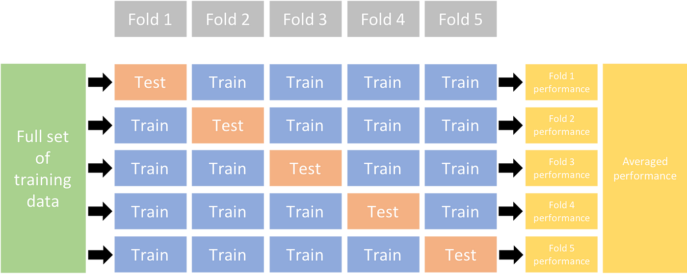
The advantage of this process is that our final cross-validated metric for our proposed pipeline is in fact the average of five different values - so even if one of the test sets is “unlucky”, the others will average it out.

Note

Remember that ultimately, all of this effort has only one goal: to get a “fair” measurement of how good a particular pipeline is at predicting, so that we can choose our best final pipeline from among the many options.

13.3.1 `cross_val_score`

Even if you are convinced that cross-validation could be useful, it might seem daunting. Imagine needing to create five different test/training sets, and go through the process of fitting, predicting, and computing metrics for every single one.

Fortunately, now that we have Pipeline objects, sklearn has shortcuts.

from sklearn.model_selection import cross_val_score

X = ames.drop("SalePrice", axis = 1)
y = ames["SalePrice"]


ct = ColumnTransformer(
  [
    ("dummify", OneHotEncoder(sparse_output = False), ["Bldg Type"]),
    ("standardize", StandardScaler(), ["Gr Liv Area", "TotRms AbvGrd"])
  ],
  remainder = "drop"
)

lr_pipeline_1 = Pipeline(
  [("preprocessing", ct),
  ("linear_regression", LinearRegression())]
).set_output(transform="pandas")


scores = cross_val_score(lr_pipeline_1, X, y, cv=5, scoring='r2')
scores

array([0.53184383, 0.53247653, 0.42905573, 0.56571819, 0.60646427])

Wow! Once the pipeline is set up, only one small line of code performs the entire cross-validation procedure!

Notice that here, we never used train_test_split(). We simply passed our entire X and y objects to the cross_val_score function, and it took care of making the 5 cross validation folds; as well as all of the fitting, predicting, and computing of metrics.

We now can simply report our final cross-validated R-squared value:

scores.mean()

0.5331117091273414

Practice Activity

Once again consider four modeling options for house price:

Using only the size and number of rooms.
Using size, number of rooms, and building type.
Using size and building type, and their interaction.
Using a 5-degree polynomial on size, a 5-degree polynomial on number of rooms, and also building type.

Use cross_val_score with the pipelines you made earlier to find the cross-validated root mean squared error for each model.

Which do you prefer? Does this agree with your conclusion from earlier?

13.3.2 Tuning

In our previous exercise, we considered one-degree polynomials as well as 5-degree polynomials. But what if we wanted to try everything from 1-degree to 10-degree, without needing to manually create 10 different pipelines?

This process - where we want to try a range of different values in our model specification and see which has the best cross-validation metrics - is called tuning.

Since tuning is a common need in modeling, sklearn has another shortcut for us, grid_search_cv. But in order to capture the process, this function needs to know:

What pipeline structure you want to try.
Which piece of the pipeline you are plugging in a range of different values for.
Which values to plug in.

We’ll start by writing ourselves a function that makes the pipeline we need for a particular degree number.

from sklearn.model_selection import GridSearchCV

ct_poly = ColumnTransformer(
  [
    ("dummify", OneHotEncoder(sparse_output = False), ["Bldg Type"]),
    ("polynomial", PolynomialFeatures(), ["Gr Liv Area"])
  ],
  remainder = "drop"
)

lr_pipeline_poly = Pipeline(
  [("preprocessing", ct_poly),
  ("linear_regression", LinearRegression())]
).set_output(transform="pandas")

degrees = {'preprocessing__polynomial__degree': np.arange(1, 10)}

gscv = GridSearchCV(lr_pipeline_poly, degrees, cv = 5, scoring='r2')

A few important things to notice in this code:

In the polynomial step of our ColumnTransformer, we did not specify the number of features in the PolynomialFeatures() function.
We created a dictionary object named degrees, which was simply a list of the numbers we wanted to try inserting into the PolynomialFeatures() function.
The name of the list of numbers in our dictionary object was preprocessing__polynomial__degree. This follows the pattern

[name of step in pipeline]__[name of step in column transformer]__[name of argument to function]

The code above did not result in cross-validated metrics for the 9 model options (degrees 1 to 9). Like a Pipeline object, a GridSearchCV object “sets up” a process - we haven’t actually given it data yet.

Note

You might be noticing a pattern in sklearn here: in general (although not always), a capitalized function is a “set up” step, like LinearRegression() or OneHotEncoder or Pipeline(). A lowercase function is often a calculation on data, like .fit() or .predict() or cross_val_score().

Now, we will fit our “grid search” tuning procedure to the data:

gscv_fitted = gscv.fit(X, y)

gscv_fitted.cv_results_

{'mean_fit_time': array([0.00373011, 0.0035553 , 0.00363498, 0.00373187, 0.00346799,
       0.00376768, 0.00669088, 0.00375037, 0.00373635]), 'std_fit_time': array([3.38883354e-04, 9.75645415e-05, 2.30070218e-04, 1.75824584e-04,
       1.73586763e-04, 3.46568232e-04, 5.88991242e-03, 8.52224735e-05,
       8.85113811e-05]), 'mean_score_time': array([0.00158796, 0.00151463, 0.00150099, 0.00152459, 0.0014884 ,
       0.00157409, 0.00168405, 0.00159721, 0.00150619]), 'std_score_time': array([1.71109784e-04, 6.70866670e-05, 1.43201241e-04, 7.17739878e-05,
       1.24161236e-04, 9.94328850e-05, 2.57057937e-04, 1.00324816e-04,
       2.26392722e-05]), 'param_preprocessing__polynomial__degree': masked_array(data=[1, 2, 3, 4, 5, 6, 7, 8, 9],
             mask=[False, False, False, False, False, False, False, False,
                   False],
       fill_value='?',
            dtype=object), 'params': [{'preprocessing__polynomial__degree': 1}, {'preprocessing__polynomial__degree': 2}, {'preprocessing__polynomial__degree': 3}, {'preprocessing__polynomial__degree': 4}, {'preprocessing__polynomial__degree': 5}, {'preprocessing__polynomial__degree': 6}, {'preprocessing__polynomial__degree': 7}, {'preprocessing__polynomial__degree': 8}, {'preprocessing__polynomial__degree': 9}], 'split0_test_score': array([0.53667199, 0.53861812, 0.55155397, 0.55000299, 0.50847886,
       0.50803388, 0.50404864, 0.48824759, 0.45353318]), 'split1_test_score': array([0.52379929, 0.51739889, 0.52489524, 0.52536327, 0.45451042,
       0.45231332, 0.44389116, 0.42226201, 0.38464169]), 'split2_test_score': array([  0.43205901,   0.44999102,   0.50538581,   0.45008921,
         0.1733882 ,  -0.39418512,  -1.67096399,  -4.78706736,
       -12.6045523 ]), 'split3_test_score': array([  0.56266573,   0.57574172,   0.58653708,   0.59197747,
         0.54742275,   0.53273129,   0.31370342,  -1.49591606,
       -11.46561678]), 'split4_test_score': array([0.59424739, 0.57528078, 0.58780969, 0.59316272, 0.57550038,
       0.5702938 , 0.55592936, 0.53199328, 0.50402512]), 'mean_test_score': array([ 0.52988868,  0.5314061 ,  0.55123636,  0.54211913,  0.45186012,
        0.33383744,  0.02932172, -0.96809611, -4.54559382]), 'std_test_score': array([0.05453461, 0.04640531, 0.03280237, 0.05273277, 0.14503685,
       0.36602408, 0.85397816, 2.05754398, 6.12585788]), 'rank_test_score': array([4, 3, 1, 2, 5, 6, 7, 8, 9], dtype=int32)}

Oof, this is a lot of information!

Ultimately, what we care about is the cross-validated metric (i.e. average over the 5 folds) for each of the 9 proposed models.

gscv_fitted.cv_results_['mean_test_score']

array([ 0.52988868,  0.5314061 ,  0.55123636,  0.54211913,  0.45186012,
        0.33383744,  0.02932172, -0.96809611, -4.54559382])

It can sometimes be handy to convert these results to a pandas data frame for easy viewing:

pd.DataFrame(data = {"degrees": np.arange(1, 10), "scores": gscv_fitted.cv_results_['mean_test_score']})

   degrees    scores
0        1  0.529889
1        2  0.531406
2        3  0.551236
3        4  0.542119
4        5  0.451860
5        6  0.333837
6        7  0.029322
7        8 -0.968096
8        9 -4.545594

It appears that the third model - degree 3 - had the best cross-validated metrics, with an R-squared value of about 0.55.

Check In

Recall that the model fitting step is when coefficients are computed for the linear regression.

How many different model fitting steps occurred when gscv.fit(X, y) was run?

13.3.3 Your Turn

Practice Activity

Consider one hundred modeling options for house price:

House size, trying degrees 1 through 10
Number of rooms, trying degrees 1 through 10
Building Type

Hint: The dictionary of possible values that you make to give to GridSearchCV will have two elements instead of one.

Q1: Which model performed the best?

Q2: What downsides do you see of trying all possible model options? How might you go about choosing a smaller number of tuning values to try?

13.1 Introduction

13.2 Pipelines

13.2.1 Cautionary Tale:

13.2.1.1 Chapter One

13.2.1.2 Chapter Two

13.2.1.3 The Moral of the Story

13.2.2 Pipeline Objects

13.2.3 Column Transformers

13.2.3.1 Checking preprocessing

13.2.4 Challenges of pipelines

13.2.4.1 Extracting information

13.2.4.2 Pandas input, numpy output

13.2.4.3 Interactions and Dummies

13.2.5 Your turn

13.3 Cross-Validation

13.3.1 cross_val_score

13.3.2 Tuning

13.3.3 Your Turn

13.3.1 `cross_val_score`