import pandas as pd
from palmerpenguins import load_penguins
from plotnine import ggplot, geom_point, aes, geom_boxplot3 Data Visualization in Python
3.1 Introduction
This document demonstrates the use of the plotnine library in Python to visualize data via the grammar of graphics framework.
The functions in plotnine originate from the ggplot2 R package, which is the R implementation of the grammar of graphics.
3.2 Grammar of Graphics
The grammar of graphics is a framework for creating data visualizations.
A visualization consists of:
The aesthetic: Which variables are dictating which plot elements.
The geometry: What shape of plot your are making.
For example, the plot below displays some of the data from the Palmer Penguins data set.
First, though, we need to load the Palmer Penguins dataset.
Note
If you do not have the pandas library installed then you will need to run
pip install pandas
in the Jupyter terminal to install. Same for any other libraries you haven’t installed.
penguins = load_penguins()

(ggplot(penguins, aes(x = "species", y = "bill_length_mm", fill = "species"))
+ geom_boxplot()
)
<Figure Size: (640 x 480)>
The aesthetic is species on the x-axis, bill_length_mm on the y-axis, colored by species.
The geometry is a boxplot.
3.3 plotnine (i.e. ggplot)
The plotnine library implements the grammar of graphics in Python.
Code for the previous example:
(ggplot(penguins, aes(x = "species", y = "bill_length_mm", fill = "species"))
+ geom_boxplot()
)
3.3.1 The aesthetic
(ggplot(penguins,
1aes(
2  x = "species",
  y = "bill_length_mm",
  fill = "species"))
+ geom_boxplot()
)- 1
-
The
aes()function is the place to specify aesthetics. - 2
-
x,y, andfillare three possible aesthetics that can be specified, that map variables in our data set to plot elements.
<Figure Size: (640 x 480)>
3.3.2 The geometry
(ggplot(penguins,
aes(
  x = "species",
  y = "bill_length_mm",
  fill = "species"))
1+ geom_boxplot()
)- 1
-
A variety of
geom_*functions allow for different plotting shapes (e.g. boxplot, histogram, etc.)
<Figure Size: (640 x 480)>
3.3.3 Other optional elements:
The scales of the x- and y-axes.
The color of elements that are not mapped to aesthetics.
The theme of the plot
…and many more!
3.3.4 Scales
(ggplot(penguins, aes(x = "species", y = "bill_length_mm", fill = "species"))
+ geom_boxplot()
)
<Figure Size: (640 x 480)>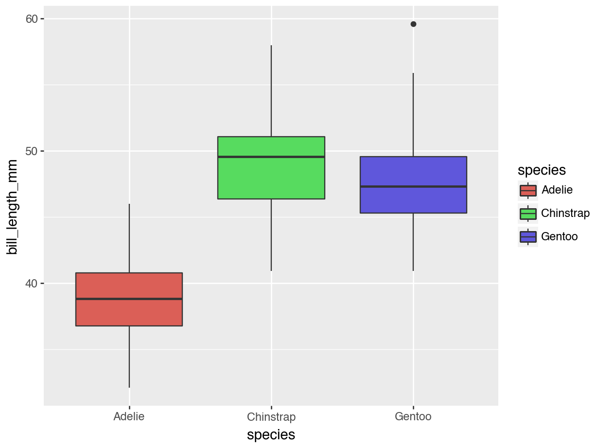
versus
from plotnine import scale_y_reverse
(ggplot(penguins, aes(x = "species", y = "bill_length_mm", fill = "species"))
+ geom_boxplot()
+ scale_y_reverse()
)
<Figure Size: (640 x 480)>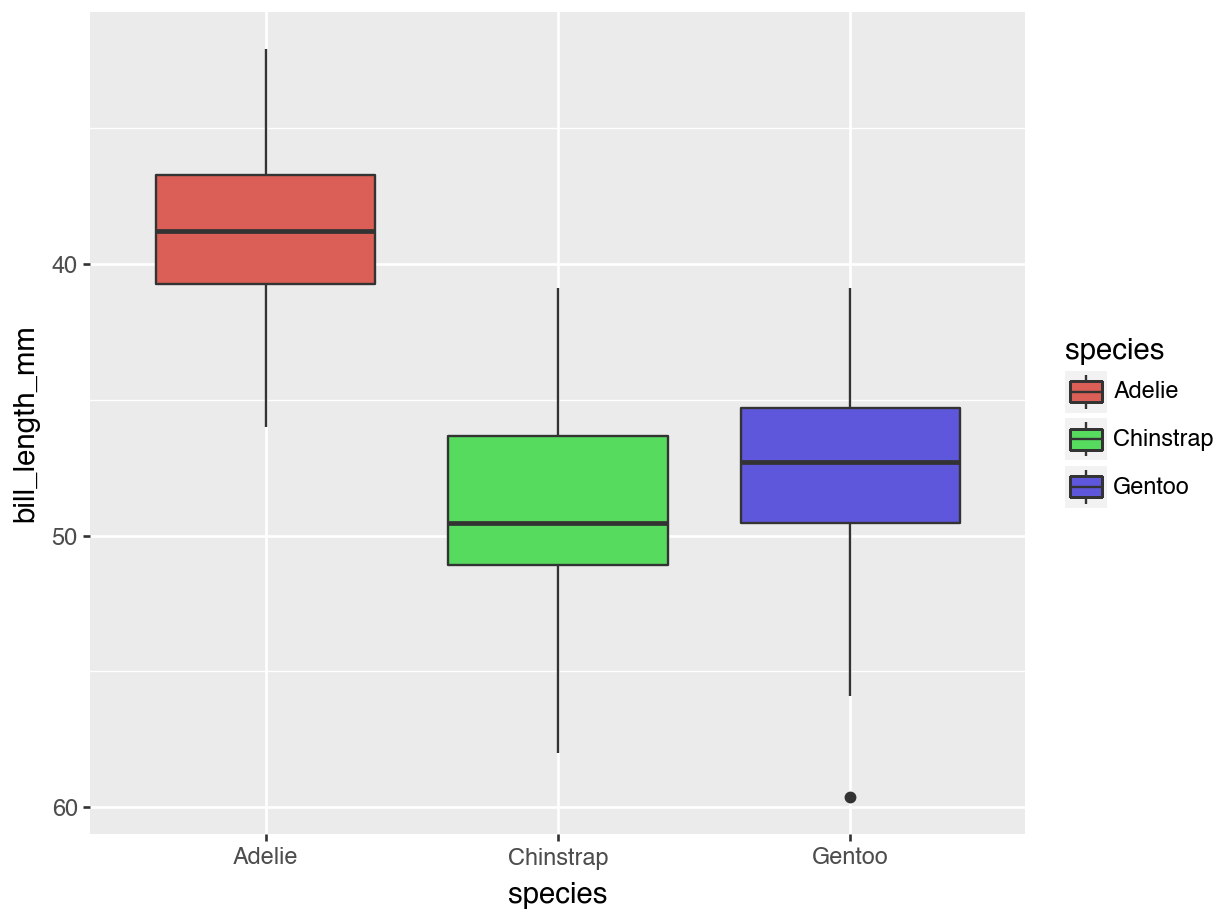
3.3.5 Non-aesthetic colors
(ggplot(penguins, aes(x = "species", y = "bill_length_mm", fill = "species"))
+ geom_boxplot()
)
<Figure Size: (640 x 480)>
versus
(ggplot(penguins, aes(x = "species", y = "bill_length_mm", fill = "species"))
+ geom_boxplot(fill = "cornflowerblue")
)
<Figure Size: (640 x 480)>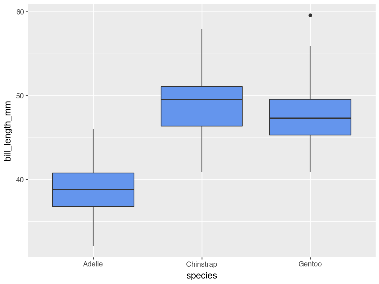
(ggplot(penguins,
aes(
  x = "species",
  y = "bill_length_mm",
  fill = "cornflowerblue"))
+ geom_boxplot()
)
3.3.6 Themes
(ggplot(penguins, aes(x = "species", y = "bill_length_mm", fill = "species"))
+ geom_boxplot()
)
<Figure Size: (640 x 480)>
versus
from plotnine import theme_classic
(ggplot(penguins, aes(x = "species", y = "bill_length_mm", fill = "species"))
+ geom_boxplot()
+ theme_classic()
)
<Figure Size: (640 x 480)>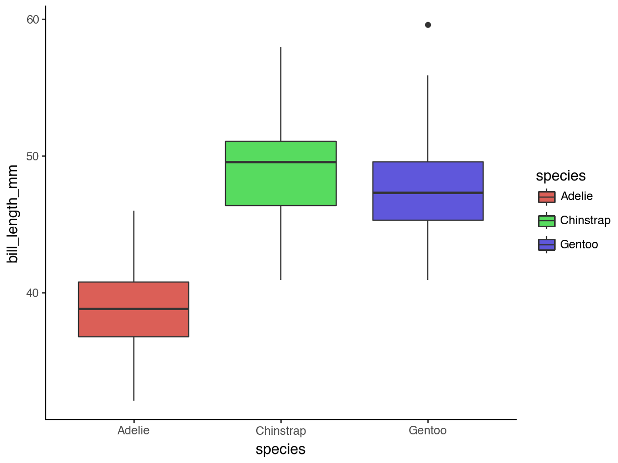
Check In
What are the aesthetics, geometry, scales, and other options in the cartoon plot below?
3.4 Geometries: The “Big Five”
3.4.1 1. Bar Plots
Most often used for showing counts of a categorical variable:
from plotnine import geom_bar
(ggplot(penguins,
aes(
  x = "species"
))
+ geom_bar()
)
<Figure Size: (640 x 480)>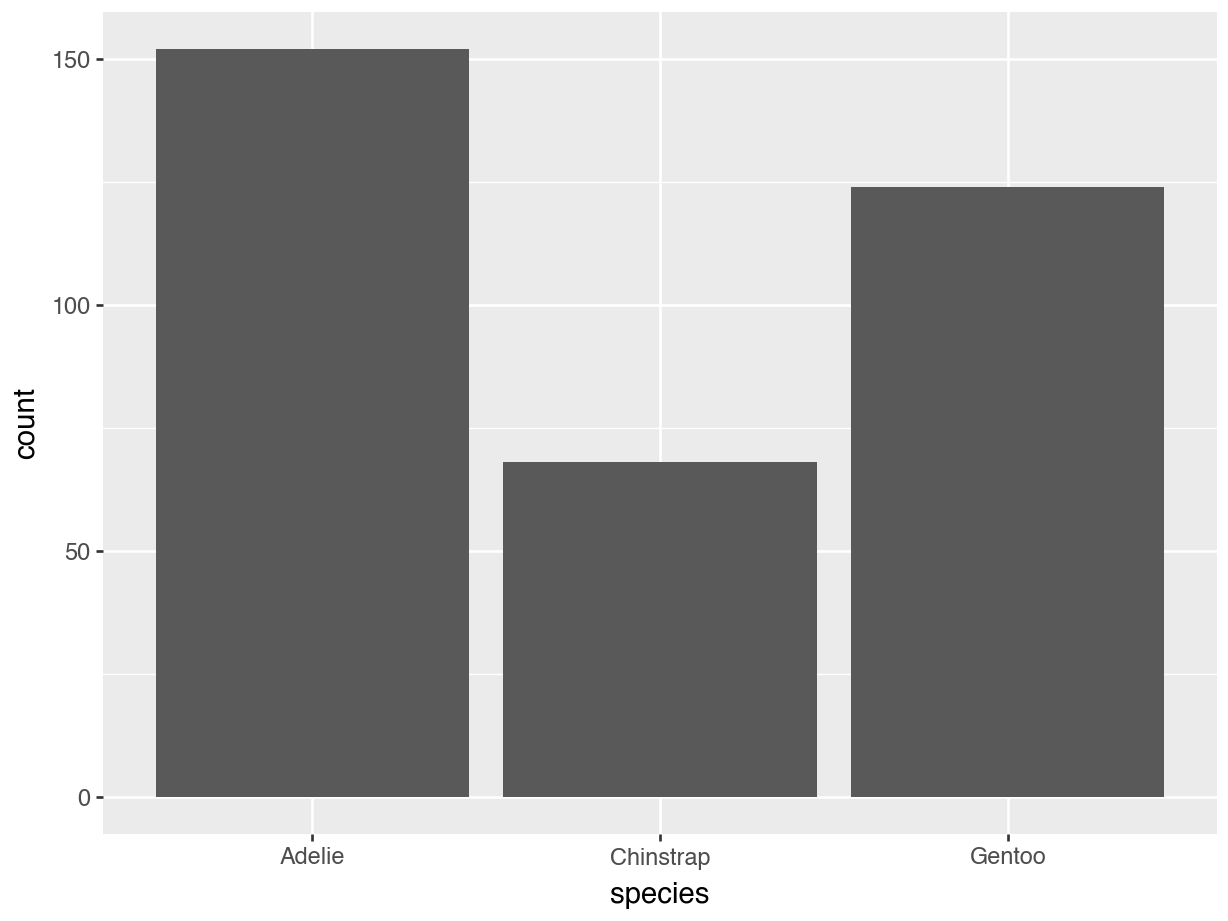
… or relationships between two categorical variables:
(ggplot(penguins,
aes(
  x = "species",
  fill = "sex"
))
+ geom_bar()
)
<Figure Size: (640 x 480)>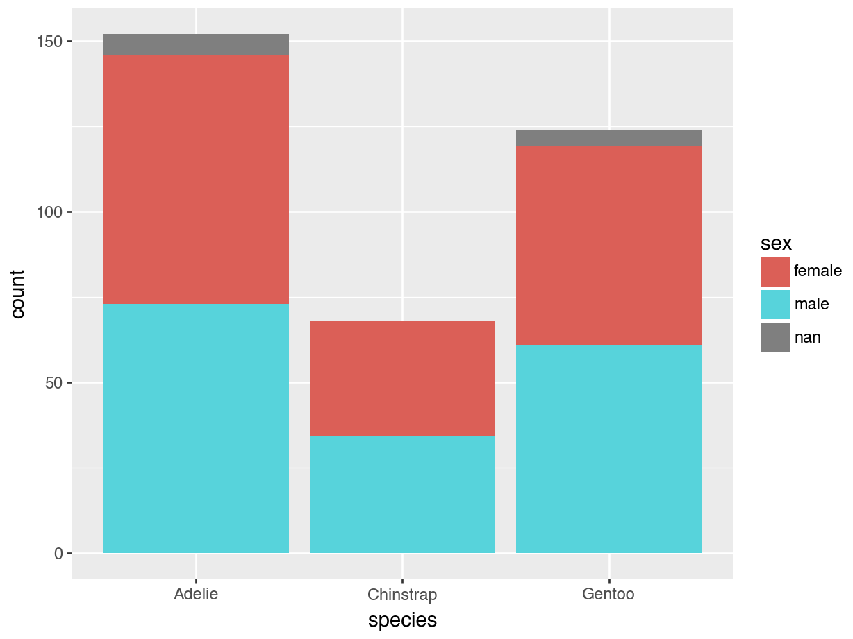
Would we rather see percents?
(ggplot(penguins,
aes(
  x = "species",
  fill = "island"
))
+ geom_bar(position = "fill")
)
<Figure Size: (640 x 480)>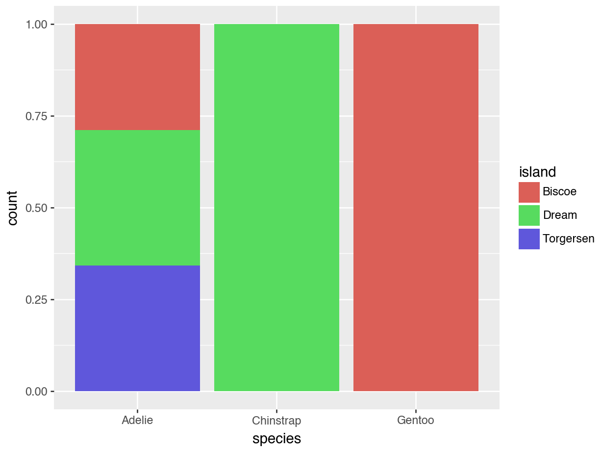
Or side-by-side?
(ggplot(penguins,
aes(
  x = "species",
  fill = "island"
))
+ geom_bar(position = "dodge")
)
<Figure Size: (640 x 480)>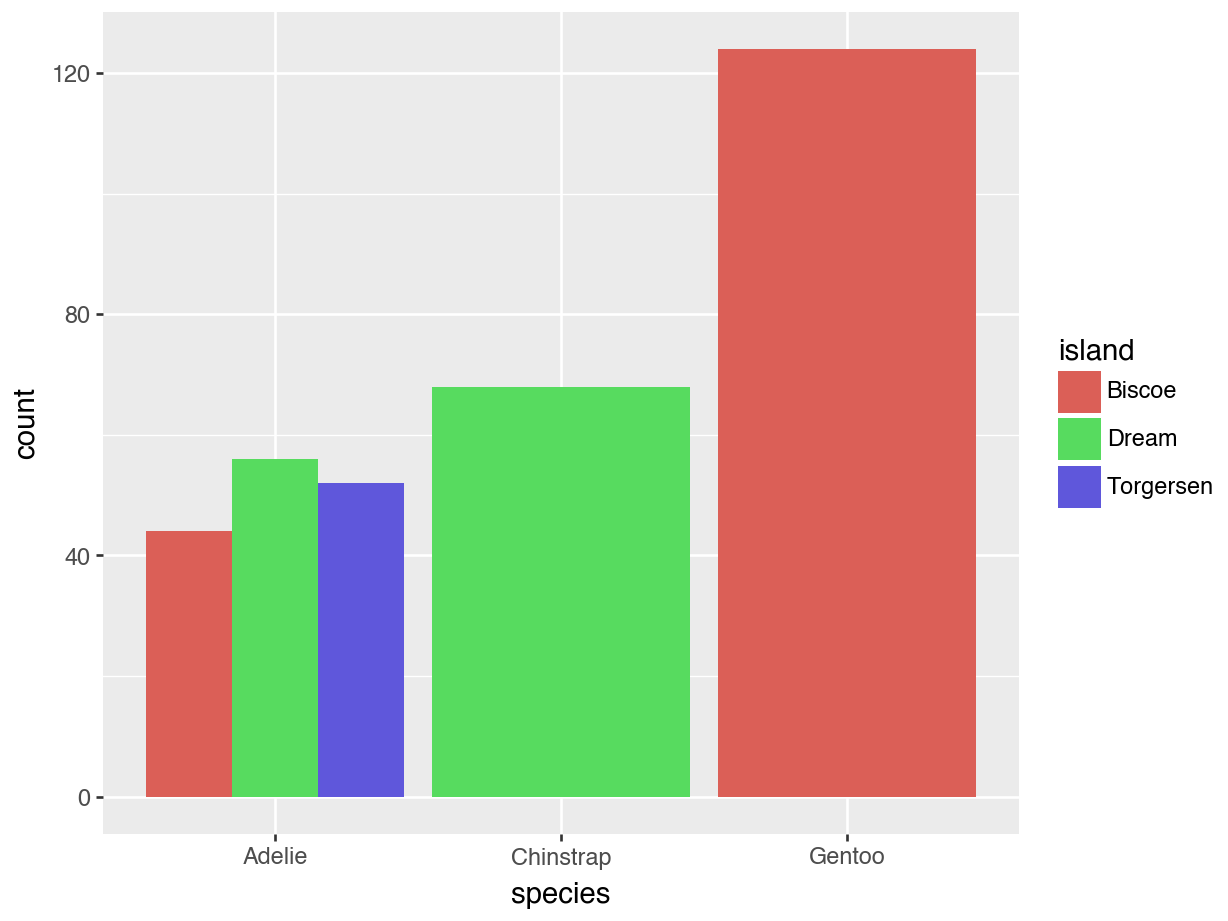
3.4.2 2. Boxplots
(ggplot(penguins,
aes(
  x = "species",
  y = "bill_length_mm"
))
+ geom_boxplot()
)
<Figure Size: (640 x 480)>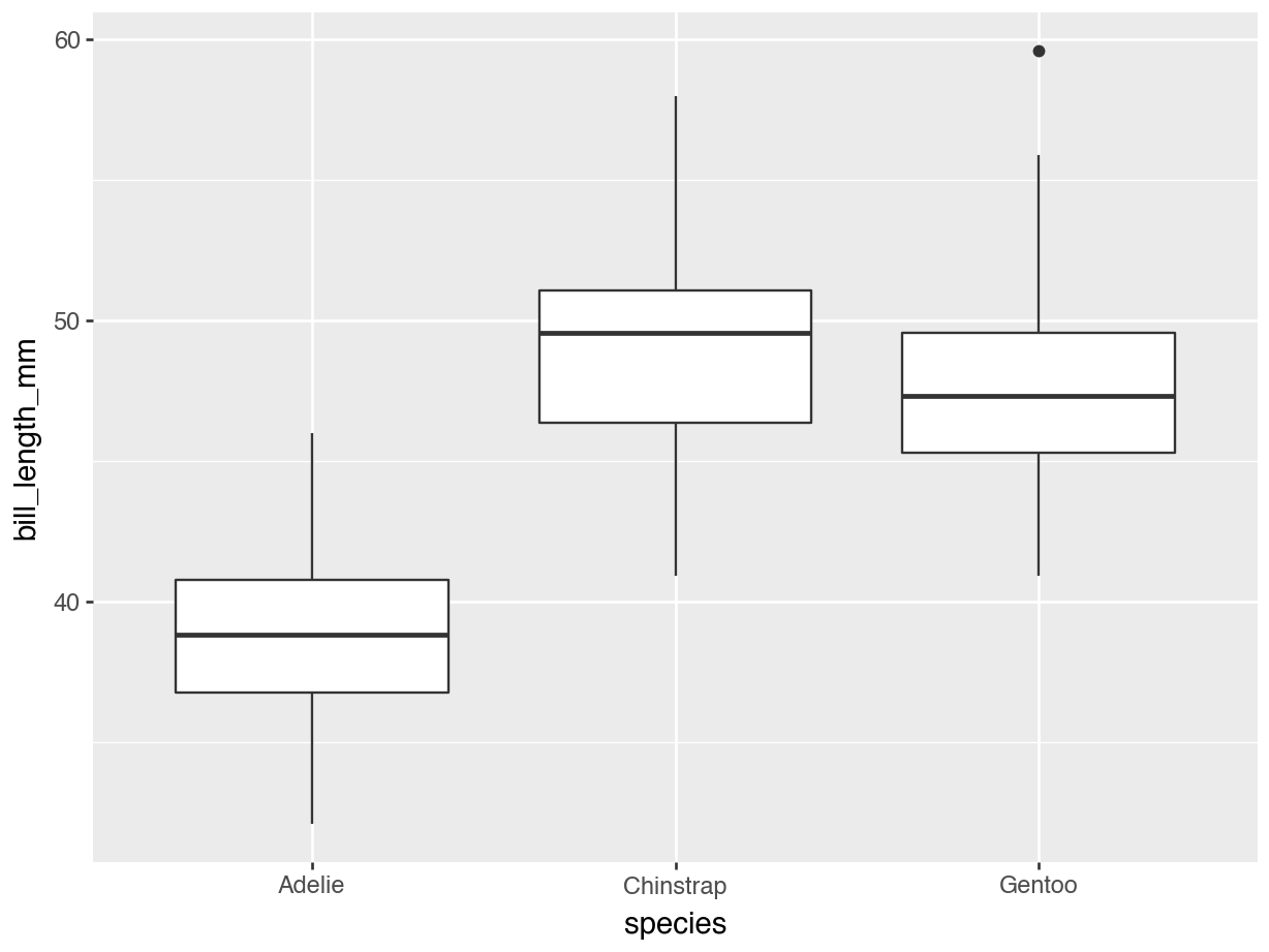
Side-by-side using a categorical variable:
(ggplot(penguins,
aes(
  x = "species",
  y = "bill_length_mm",
  fill = "sex"
))
+ geom_boxplot()
)
<Figure Size: (640 x 480)>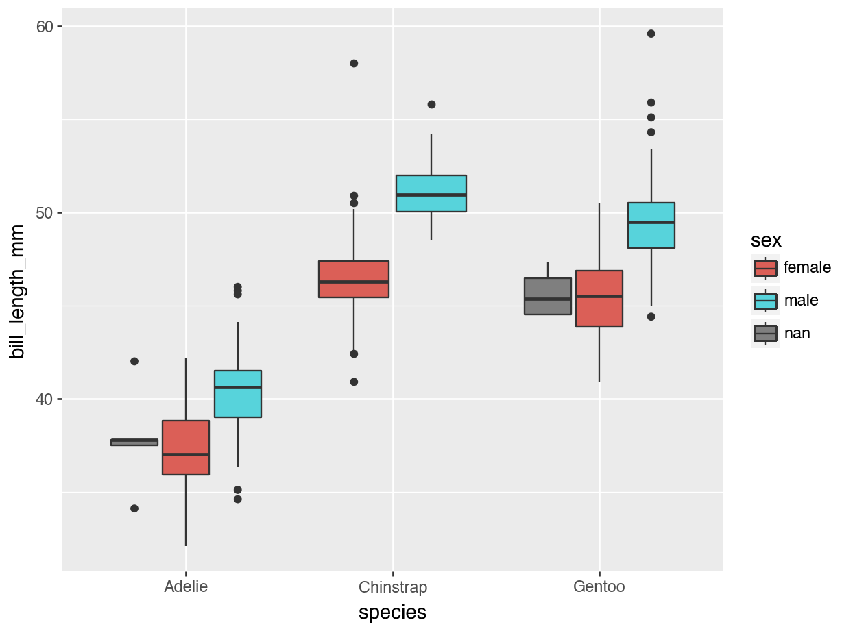
3.4.3 3. Histograms
from plotnine import geom_histogram
(ggplot(penguins,
aes(
  x = "bill_length_mm"
))
+ geom_histogram()
)
<Figure Size: (640 x 480)>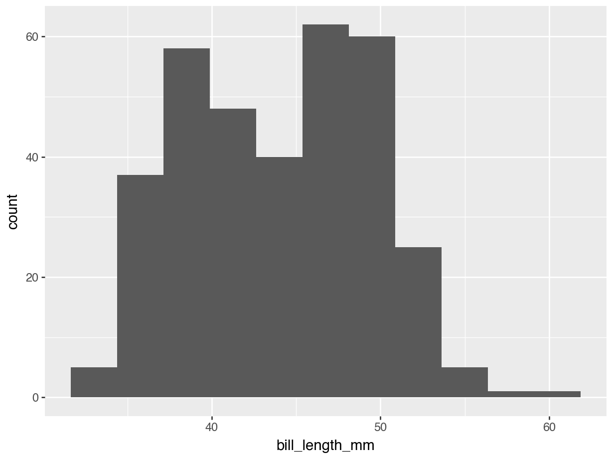
(ggplot(penguins,
aes(
  x = "bill_length_mm"
))
+ geom_histogram(bins = 100)
)
<Figure Size: (640 x 480)>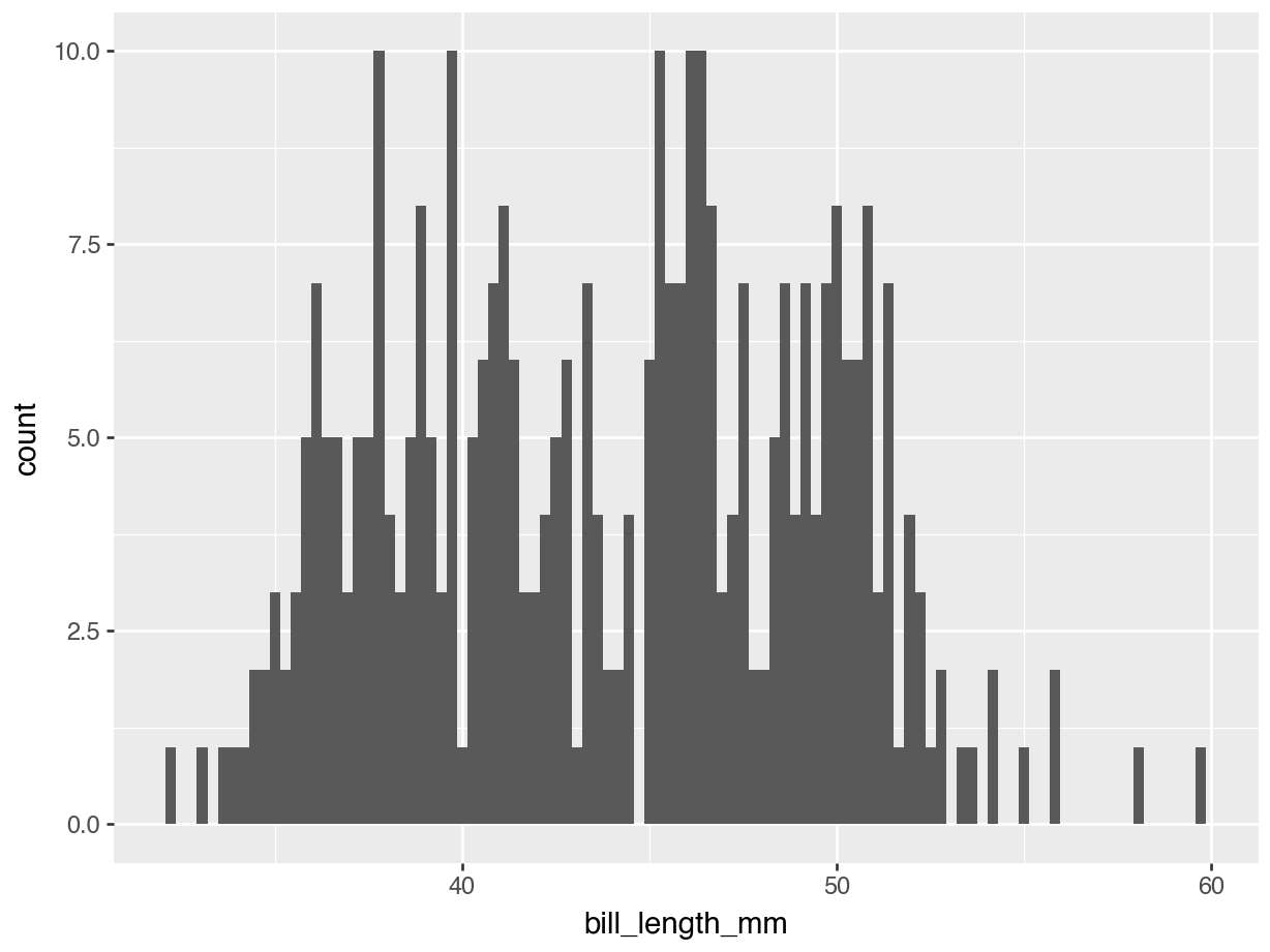
(ggplot(penguins,
aes(
  x = "bill_length_mm"
))
+ geom_histogram(bins = 10)
)
<Figure Size: (640 x 480)>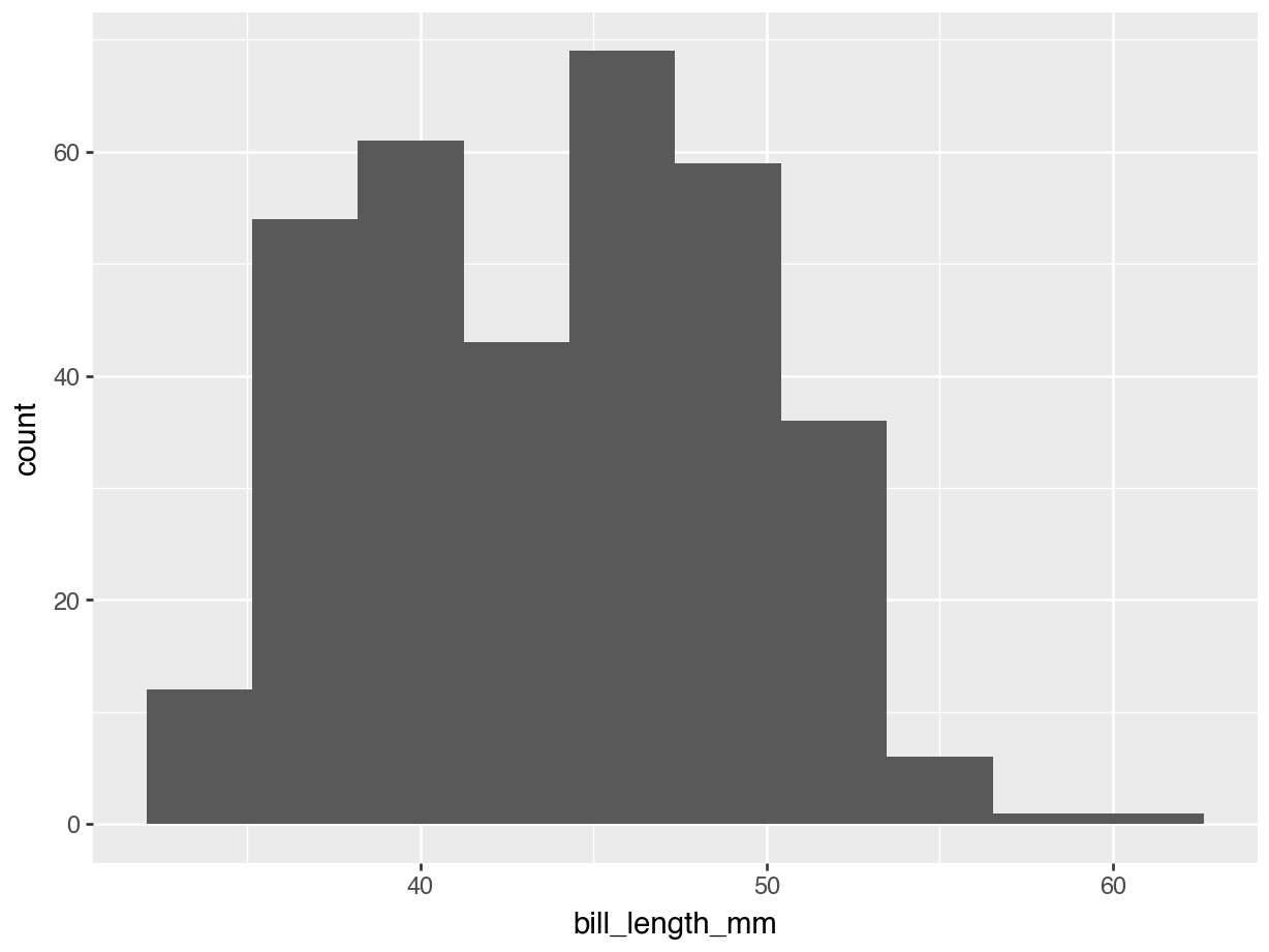
3.4.4 3.5 Densities
Suppose you want to compare histograms by category:
(ggplot(penguins,
aes(
  x = "bill_length_mm",
  fill = "species"
))
+ geom_histogram()
)
<Figure Size: (640 x 480)>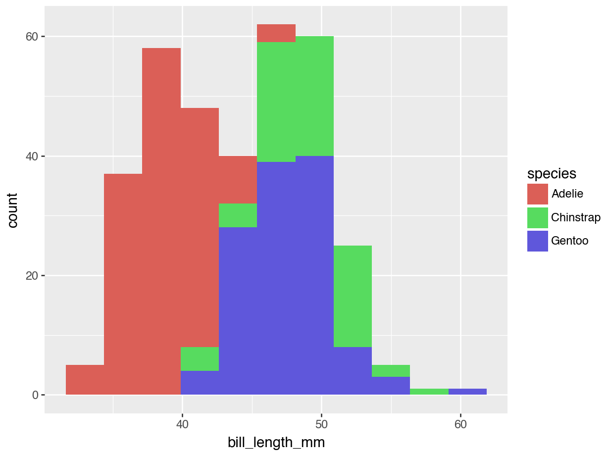
Cleaner: smoothed histogram, or density:
from plotnine import geom_density
(ggplot(penguins,
aes(
  x = "bill_length_mm",
  fill = "species"
))
+ geom_density()
)
<Figure Size: (640 x 480)>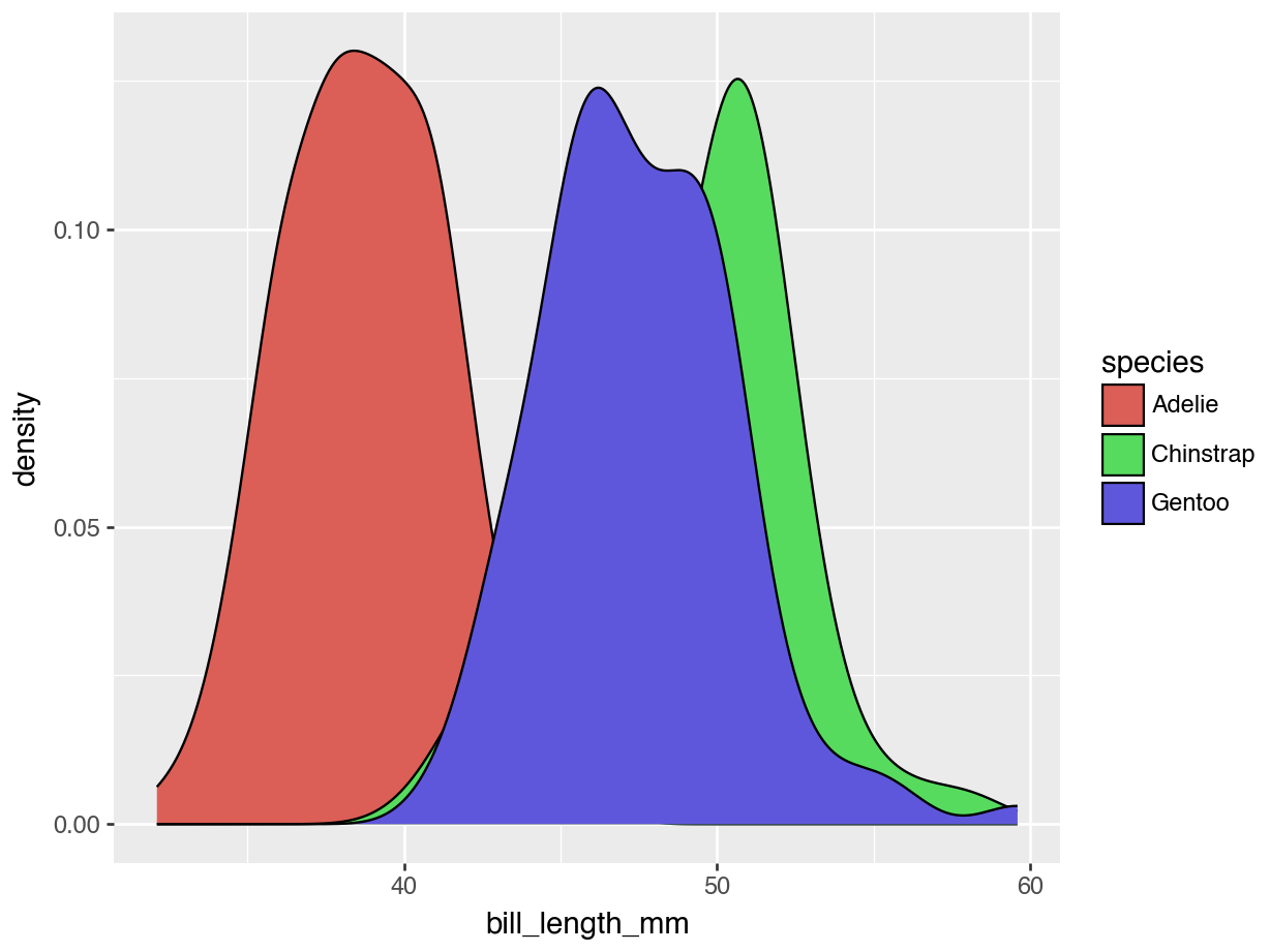
Even cleaner: The alpha option:
(ggplot(penguins,
aes(
  x = "bill_length_mm",
  fill = "species"
))
+ geom_density(alpha = 0.5)
)
<Figure Size: (640 x 480)>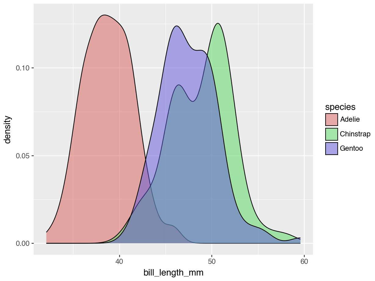
3.4.5 4. Scatterplots
(ggplot(penguins,
aes(
  x = "bill_length_mm",
  y = "bill_depth_mm"
))
+ geom_point()
)
<Figure Size: (640 x 480)>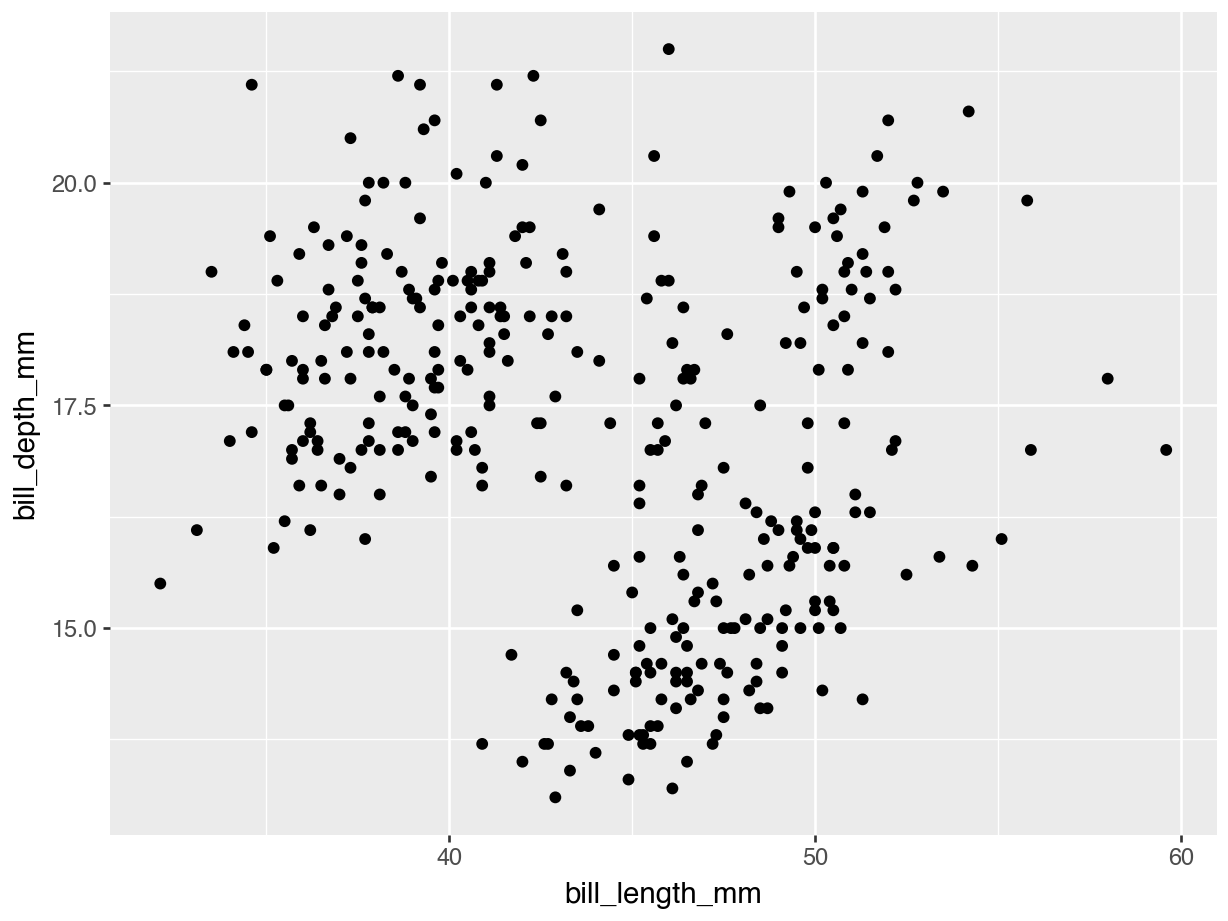
Colors for extra information:
(ggplot(penguins,
aes(
  x = "bill_length_mm",
  y = "bill_depth_mm",
  color = "species"
))
+ geom_point()
)
<Figure Size: (640 x 480)>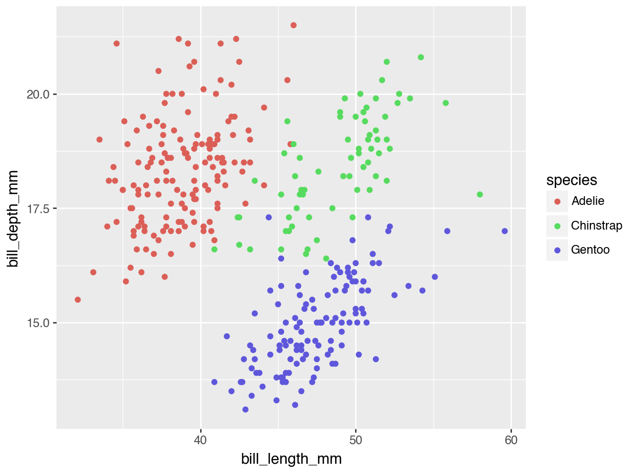
3.4.6 5. Line Plots
from plotnine import geom_line
penguins2 = penguins.groupby(["species", "sex"])[["bill_length_mm"]].mean().reset_index()

(ggplot(penguins2,
aes(
  x = "species",
  y = "bill_length_mm",
  color = "sex",
  group = "sex"
))
+ geom_point()
+ geom_line()
)
<Figure Size: (640 x 480)>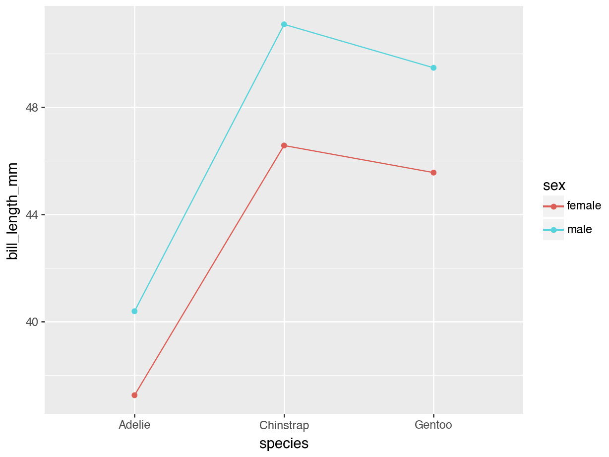
3.5 Multiple Plots
3.5.1 Facet Wrapping
from plotnine import facet_wrap
(ggplot(penguins,
aes(
  x = "species",
  y = "bill_length_mm"
))
+ geom_boxplot()
+ facet_wrap("sex")
)
<Figure Size: (640 x 480)>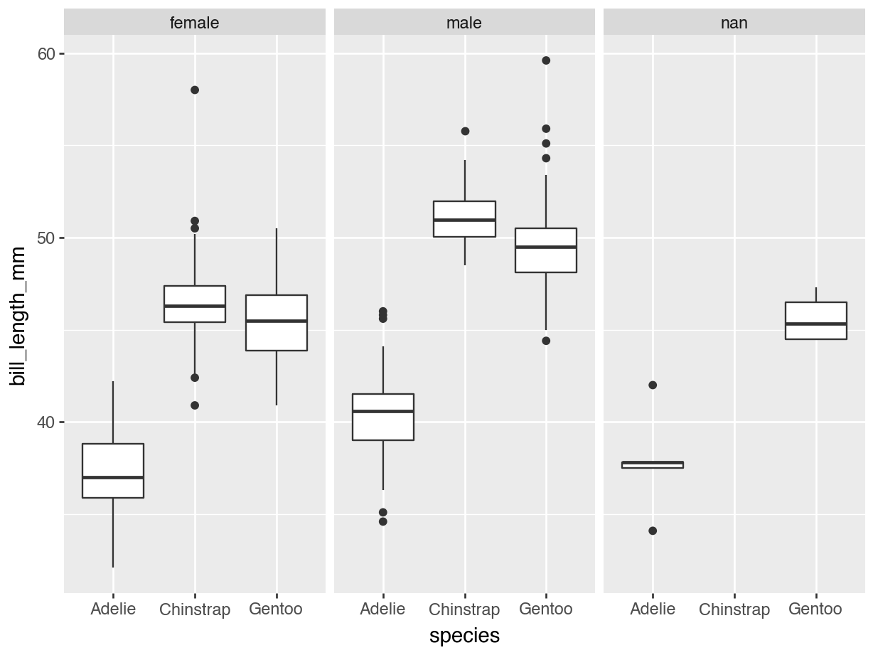
3.6 Visualization and GenAI
In our experience, generative AI can help with the data visualization process in two major ways:
3.6.1 1. Brainstorming possible visualizations for a particular research question.
Sometimes, it can be hard to imagine what a plot will look like or which geometries to use - you sink time into writing out your code, only to be disappointed when the resulting image is not as compelling as you hoped.
With careful prompting, many genAI tools can suggest plot types and then “preview” these plot ideas for you. There are some limitations, however:
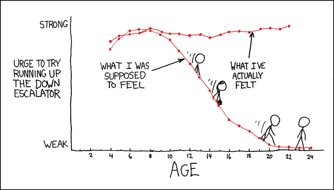
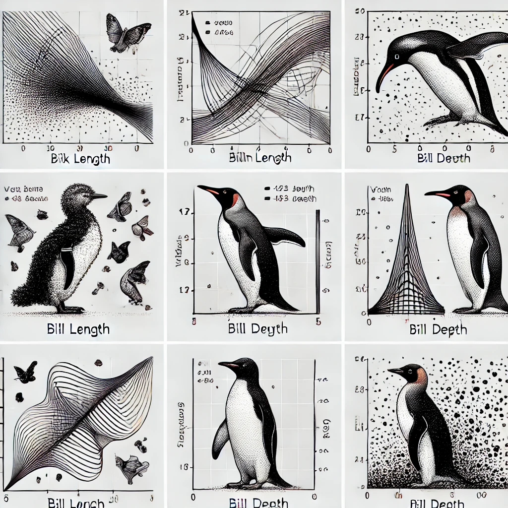
- When asking for this service, make sure to ask for the code output specifically. In one attempt to demonstrate this task, I carelessly used the phrase “sketch a plot”, and GPT-4o took the “sketch” command very seriously, as you can see below!
- The GenAI does not have access to your specific dataset. That means the tool cannot fully preview how your plots might look on your data. What it can do, though, is show comparable examples on another dataset.
The goal here is not to fully produce your final visualization. The goal is to get a general sense of what geometry options might fit your research question, and how each of those would look.
3.6.2 2. Building code layer by layer.
3.6.2.1 Initial plot
If you find it psychologically easier to edit code than to start from scratch, genAI can be very adept at producing basic visualization code for you to build on. This chat shows a very quick example.
3.6.2.2 Specific syntax to tweak your visual
Once you have your basic plot code, the genAI tool becomes an excellent reference/documentation for how to add layers and make tweaks. For example, suppose in the above example we wanted to see the bill lengths on a logarithmic scale. In this chat, we see how easily Chat GPT-4o is able to add the ggplot layer of + scale_y_log10()
3.6.2.3 Principles
Since this use of AI involves asking it to write actual code for you, remember the WEIRDER principles:
Well-specified: The more specifically we can describe our plot, the better resulting code you will get. Make sure to mention which plotting library you want to use, what geometry you are using, and what your variable mappings are.
Editable: Don’t try to get the AI tool to create your final perfect polished visualization from the first prompt; this can lead to overly complicated code that is hard to tweak. Instead, add complexity bit by bit, checking at each step for ways to improve or clarify the AI-generated code.
Interpretable: The AI tool will sometimes leap to conclusions about the plot, making unprompted changes to the titles, the scales, or the theme. Make sure you review each layer of the ggplot process, and ensure that it is indeed what you intended.
Reproducible: Sometimes, when you ask for a particular small visual change, the AI will achieve this task manually. For example, if you ask for particular labels on the x-axis, it may choose to remove all labels and put numbers in “by hand”, rather than generally changing the scale. (Look for an example of this with the facet titles in the activity at the end of this section!)
Even if the AI-generated code achieves the visual you hoped for, make sure to review the code for instances where you need to replace sloppy solutions with cleaner ones.
Dependable: The good news is, unit testing in visualization is easy: simply run the code and see if the output looks how you hoped!
Ethical: Just because an LLM suggests a visual doesn’t mean it is a responsible one. You, as the human creator, must review your visualizations to ensure they are not conveying any harmful information or impressions.
References: If you use AI-generated code in your visualization, you absolutely must state this up front in your work, even if you heavily edit the initial code.
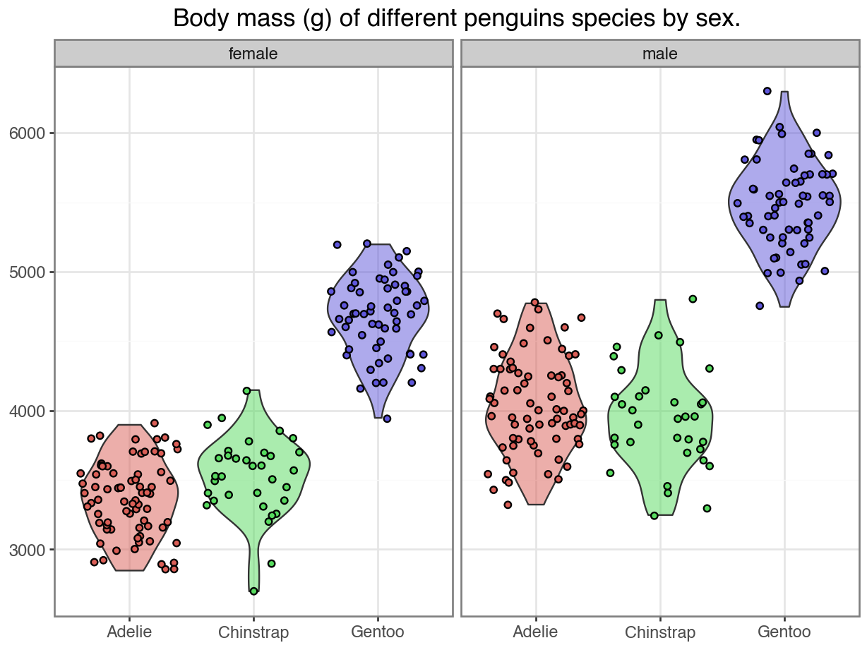
3.6.3 Try it out
Code
import pandas as pd
from palmerpenguins import load_penguins

penguins = load_penguins()

from plotnine import *

(
    ggplot(penguins.dropna(), aes(x="species", y="body_mass_g", fill="species"))
    + geom_violin(alpha=0.5)
    + geom_jitter()
    + facet_wrap("sex")
    + scale_fill_discrete(guide=None)
    + labs(x="", y="", title="Body mass (g) of different penguins species by sex.")
    + theme_bw()
)
<Figure Size: (640 x 480)>