2 Programming Basics

Objectives

In this chapter, we will review some basics of general computer programming, and how they appear in python.

We will also introduce the role of GenAI in programming and how it will be covered in this course.

Learn More

Some of you may find this material to be unneeded review - if so, great!

But if you are new to programming, or it has been a while, this tutorial may help you refresh your knowledge.

2.1 Basic Data Types

It is important to have a base grasp on the types of data you might see in data analyses.

2.1.1 Values and Types

Let’s start this section with some basic vocabulary.

a value is a basic unit of stuff that a program works with, like 1, 2, "Hello, World", and so on.
values have types - 2 is an integer, "Hello, World" is a string (it contains a “string” of letters). Strings are in quotation marks to let us know that they are not variable names.

In python, there are some very basic data types:

logical or boolean - False/True or 0/1 values. Sometimes, boolean is shortened to bool
integer - whole numbers (positive or negative)
double or float - decimal numbers.
- float is short for floating-point value.
- double is a floating-point value with more precision (“double precision”).¹
numeric - python uses the name numeric to indicate a decimal value, regardless of precision.
character or string or object - holds text, usually enclosed in quotes.

If you don’t know what type a value is, python has a function to help you with that.

type(False)
type(2) # by default, python treats whole numbers as integers
type(2.0)  # to force it not to be an integer, add a .0
type("Hello, programmer!")

str

Warning

In python, boolean values are True and False. Capitalization matters a LOT.

Other details: if we try to write a million, we would write it 1000000 instead of 1,000,000. Commas are used for separating numbers, not for proper spacing and punctuation of numbers. This is a hard thing to get used to but very important – especially when we start reading in data.

2.1.2 Variables

Programming languages use variables - names that refer to values. Think of a variable as a container that holds something - instead of referring to the value, you can refer to the container and you will get whatever is stored inside.

In python, we assign variables values using the syntax object_name = value You can read this as “object name gets value” in your head.

message = "So long and thanks for all the fish"
year = 2025
the_answer = 42
earth_demolished = False

We can then use the variables - do numerical computations, evaluate whether a proposition is true or false, and even manipulate the content of strings, all by referencing the variable by name.

message + ", sang the dolphins."

year + the_answer

not earth_demolished

True

2.1.2.1 Valid Names

There are only two hard things in Computer Science: cache invalidation and naming things.
– Phil Karlton

Object names must start with a letter and can only contain letters, numbers, and _.

What happens if we try to create a variable name that isn’t valid?

Starting a variable name with a number will get you an error message that lets you know that something isn’t right.

1st_thing = "No starting with numbers"

first~thing = "No other symbols"

first.thing = "Periods have a particular meaning!"

SyntaxError: invalid syntax (3761243318.py, line 1)

Naming things is difficult! When you name variables, try to make the names descriptive - what does the variable hold? What are you going to do with it? The more (concise) information you can pack into your variable names, the more readable your code will be.

Learn More

Why is naming things hard? - Blog post by Neil Kakkar

There are a few different conventions for naming things that may be useful:

some_people_use_snake_case, where words are separated by underscores
somePeopleUseCamelCase, where words are appended but anything after the first word is capitalized (leading to words with humps like a camel).
A few people mix conventions with variables_thatLookLike_this and they are almost universally hated.

As long as you pick ONE naming convention and don’t mix-and-match, you’ll be fine. It will be easier to remember what you named your variables (or at least guess) and you’ll have fewer moments where you have to go scrolling through your script file looking for a variable you named.

2.1.3 Type Conversions

We talked about values and types above, but skipped over a few details because we didn’t know enough about variables. It’s now time to come back to those details.

What happens when we have an integer and a numeric type and we add them together? Hopefully, you don’t have to think too hard about what the result of 2 + 3.5 is, but this is a bit more complicated for a computer for two reasons: storage, and arithmetic.

In days of yore, programmers had to deal with memory allocation - when declaring a variable, the programmer had to explicitly define what type the variable was. This tended to look something like the code chunk below:

int a = 1
double b = 3.14159

Typically, an integer would take up 32 bits of memory, and a double would take up 64 bits, so doubles used 2x the memory that integers did. R is dynamically typed, which means you don’t have to deal with any of the trouble of declaring what your variables will hold - the computer automatically figures out how much memory to use when you run the code. So we can avoid the discussion of memory allocation and types because we’re using higher-level languages that handle that stuff for us².

But the discussion of types isn’t something we can completely avoid, because we still have to figure out what to do when we do operations on things of two different types - even if memory isn’t a concern, we still have to figure out the arithmetic question.

So let’s see what happens with a couple of examples, just to get a feel for type conversion (aka type casting or type coercion), which is the process of changing an expression from one data type to another.

type(2 + 3.14159) # add integer 2 and pi
type(2 + True) # add integer 2 and TRUE
type(True + False) # add TRUE and FALSE

int

All of the examples above are ‘numeric’ - basically, a catch-all class for things that are in some way, shape, or form numbers. Integers and decimal numbers are both numeric, but so are logicals (because they can be represented as 0 or 1).

You may be asking yourself at this point why this matters, and that’s a decent question. We will eventually be reading in data from spreadsheets and other similar tabular data, and types become very important at that point, because we’ll have to know how python handles type conversions.

Check In

Do a bit of experimentation - what happens when you try to add a string and a number? Which types are automatically converted to other types? Fill in the following table in your notes:

Adding a ___ and a ___ produces a ___:

Logical	Integer	Decimal	String
Logical
Integer
Decimal
String

Above, we looked at automatic type conversions, but in many cases, we also may want to convert variables manually, specifying exactly what type we’d like them to be. A common application for this in data analysis is when there are “NA” or ” ” or other indicators in an otherwise numeric column of a spreadsheet that indicate missing data: when this data is read in, the whole column is usually read in as character data. So we need to know how to tell python that we want our string to be treated as a number, or vice-versa.

In python, we can explicitly convert a variable’s type using functions (int, float, str, etc.).

x = 3
y = "3.14159"

x + y

x + float(y)

TypeError: unsupported operand type(s) for +: 'int' and 'str'

2.2 Operators and Functions

In addition to variables, functions are extremely important in programming.

Let’s first start with a special class of functions called operators. You’re probably familiar with operators as in arithmetic expressions: +, -, /, *, and so on.

Here are a few of the most important ones:

Operation	python symbol
Addition	`+`
Subtraction	`-`
Multiplication	`*`
Division	`/`
Integer Division	`//`
Modular Division	`%`
Exponentiation	`**`

Note that integer division is the whole number answer to A/B, and modular division is the fractional remainder when A/B.

So 14 // 3 would be 4, and 14 % 3 would be 2.

14 // 3
14 % 3

Note that these operands are all intended for scalar operations (operations on a single number) - vectorized versions, such as matrix multiplication, are somewhat more complicated.

2.2.1 Order of Operations

python operates under the same mathematical rules of precedence that you learned in school. You may have learned the acronym PEMDAS, which stands for Parentheses, Exponents, Multiplication/Division, and Addition/Subtraction. That is, when examining a set of mathematical operations, we evaluate parentheses first, then exponents, and then we do multiplication/division, and finally, we add and subtract.

(1+1)**(5-2) # 2 ^ 3 = 8
1 + 2**3 * 4 # 1 + (8 * 4)
3*1**3 # 3 * 1

2.2.2 String Operations

The + operator also works on strings. Just remember that python doesn’t speak English - it neither knows nor cares if your strings are words, sentences, etc. So if you want to create good punctuation or spacing, that needs to be done in the code.

greeting = "howdy"
person = "pardner"

greeting + person
greeting + ", " + person

'howdy, pardner'

2.2.3 Functions

Functions are sets of instructions that take arguments and return values. Strictly speaking, operators (like those above) are a special type of functions – but we aren’t going to get into that now.

We’re also not going to talk about how to create our own functions just yet. We only need to know how to use functions. Let’s look at the official documentation for the function round()`.

round(number, ndigits=None)

Return number rounded to ndigits precision after the decimal point. If ndigits is omitted or is None, it returns the nearest integer to its input.

This tells us that the function requires one argument, number, a number to round. You also have the option to include a second argument, ndigits, if you want to round to something other than a whole number.

When you call a function, you can either use the names of the arguments, or simply provide the information in the expected order.

By convention, we usually use names for optional arguments but not required ones.

round(number = 2.718)
round(2.718, 2)


round(2.718)
round(2.718, ndigits = 2)

2.72

Warning

The names of functions and their arguments are chosen by the developer who created them. You should never simply assume what a function or argument will do based on the name; always check documentation or try small test examples if you aren’t sure.

2.3 Data Structures

In the previous section, we discussed 4 different data types: strings/characters, numeric/double/floats, integers, and logical/booleans. As you might imagine, things are about to get more complicated.

Data structures are more complicated arrangements of information.

Homogeneous	Heterogeneous
1D	vector	list
2D	matrix	data frame
N-D	array

Methods or attributes are a special type of function that operate only on a specific data structure When using a method in python, you can use a period . to apply the function to an object.

my_nums = [1,2,3,4,5]
my_nums.sort()

Careful, though! If a function is not specifically designed to be an attribute of the structure, this . trick won’t work.

my_nums.round()

AttributeError: 'list' object has no attribute 'round'

2.3.1 Lists

A list is a one-dimensional column of heterogeneous data - the things stored in a list can be of different types.

A lego list: the bricks are all different types and colors, but they are still part of the same data structure.

x = ["a", 3, True]
x

['a', 3, True]

The most important thing to know about lists, for the moment, is how to pull things out of the list. We call that process indexing.

2.3.1.1 Indexing

Every element in a list has an index (a location, indicated by an integer position)³.

In python, we count from 0.

x = ["a", 3, True]

x[0] # This returns a list
x[0:2] # This returns multiple elements in the list

x.pop(0)

'a'

List indexing with [] will return a list with the specified elements.

To actually retrieve the item in the list, use the .pop attribute. The only downside to .pop is that you can only access one thing at a time.

We’ll talk more about indexing as it relates to vectors, but indexing is a general concept that applies to just about any multi-value object.

2.3.2 Vectors

A vector is a one-dimensional column of homogeneous data. Homogeneous means that every element in a vector has the same data type.

We can have vectors of any data type and length we want: 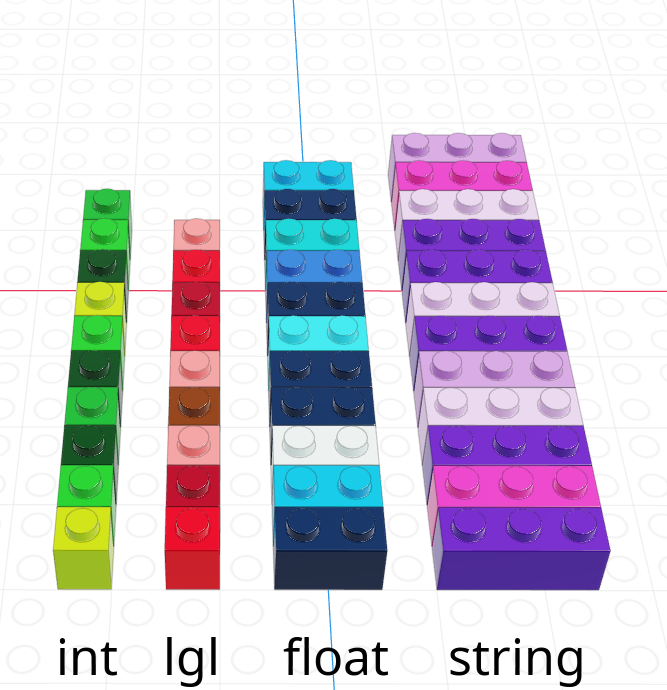vectors of different data types

Base python does not actually have a vector-type object! However, in data analysis we often have reasons to want a single-type data structure, so we will load an extra function called array from the numpy library to help us out. (More on libraries later!)

from numpy import array

digits_pi = array([3, 1, 4, 1, 5, 9, 2, 6, 5, 3, 5])

# Access individual entries
digits_pi[1]

# Print out the vector
digits_pi

array([3, 1, 4, 1, 5, 9, 2, 6, 5, 3, 5])

We can pull out items in a vector by indexing, but we can also replace specific elements as well:

favorite_cats = array(["Grumpy", "Garfield", "Jorts", "Jean"])

favorite_cats

favorite_cats[2] = "Nyan Cat"

favorite_cats

array(['Grumpy', 'Garfield', 'Nyan Cat', 'Jean'], dtype='<U8')

If you’re curious about any of these cats, see the footnotes⁴.

2.3.2.1 Boolean masking

As you might imagine, we can create vectors of all sorts of different data types. One particularly useful trick is to create a logical vector that tells us which elements of a corresponding vector we want to keep.

lego vectors - a pink/purple hued set of 1x3 bricks representing the data and a corresponding set of 1x1 grey and black bricks representing the logical index vector of the same length

If we let the black lego represent “True” and the grey lego represent “False”, we can use the logical vector to pull out all values in the main vector.

Black = True, Grey = False	Grey = True, Black = False

Note that for boolean masking to work properly, the logical index must be the same length as the vector we’re indexing. This constraint will return when we talk about data frames, but for now just keep in mind that logical indexing doesn’t make sense when this constraint isn’t true.

Example

# Define a character vector
weekdays = array(["Sunday", "Monday", "Tuesday", "Wednesday", "Thursday", "Friday", "Saturday"])
weekend = array(["Sunday", "Saturday"])

# Create logical vectors manually
relax_days = array([True, False, False, False, False, False, True])

# Create logical vectors automatically
from numpy import isin     # get a special function for arrays
relax_days = isin(weekdays, weekend) 

relax_days

# Using logical vectors to index the character vector
weekdays[relax_days] 

# Using ~ to reverse the True and False
weekdays[~relax_days]

array(['Monday', 'Tuesday', 'Wednesday', 'Thursday', 'Friday'],
      dtype='<U9')

2.3.2.2 Reviewing Types

As vectors are a collection of things of a single type, what happens if we try to make a vector with differently-typed things?

Example

array([2, False, 3.1415, "animal"]) # all converted to strings

array([2, False, 3.1415]) # converted to numerics

array([2, False]) # converted to integers

array([2, 0])

As a reminder, this is an example of implicit type conversion - python decides what type to use for you, going with the type that doesn’t lose data but takes up as little space as possible.

Warning

Implicit type conversions may seem convenient, but they are dangerous! Imagine that you created one of the arrays above, expecting it to be numeric, and only found out later that python had made it into strings.

2.3.3 Matrices

A matrix is the next step after a vector - it’s a set of values arranged in a two-dimensional, rectangular format.

lego depiction of a 3-row, 4-column matrix of 2x2 red-colored blocks

Once again, we need to use the numpy package to allow the matrix type to exist in python.

from numpy import matrix

matrix([[1,2,3], [4,5,6]])

matrix([[1, 2, 3],
        [4, 5, 6]])

Note

Notice how we give the matrix() function an argument that is a “list of lists”. That is, the first item in the list is [1,2,3] which is itself a list.

You can always think of lists as the most “neutral” data structure - if you don’t know what you want to use, it’s reasonably to start with the list, and then adjust from there, as we have with the array() and matrix() functions from numpy.

2.3.3.1 Indexing in Matrices

python uses [row, column] to index matrices. To extract the bottom-left element of a 3x4 matrix, we would use [2,0] to get to the third row and first column entry (remember that Python is 0-indexed).

As with vectors, you can replace elements in a matrix using assignment.

Example

my_mat = matrix([[1,2,3,4], [4,5,6,7], [7,8,9,10]])

my_mat

my_mat[2,0] = 500

my_mat

matrix([[  1,   2,   3,   4],
        [  4,   5,   6,   7],
        [500,   8,   9,  10]])

We will not use matrices often in this class, but there are many math operations that are very specific to matrices. If you continue on in your data science journey, you will probably eventually need to do matrix algebra in python.

Learn More

Tutorial: Linear Algebra in python

2.4 Libraries and Open-Source

2.4.1 Open-source languages

One of the great things about python is that it is an open-source language. This means that it was and is developed by individuals in a community rather than a private company, and the core code of it is visible to everyone.

The major consequences are:

It is free for anyone to use, rather than behind a paywall. (SAS or Java are examples of languages produced by private companies that require paid licenses to use.)
The language grows quickly, and in many diverse ways, because anyone at all can write their own programs. (You will write functions in a couple weeks!)
You are not allowed to sell your code for profit. (You can still write private code to help your company with a task - but you may not charge money to others for the programs themselves.)

Just our opinion...

We believe very strongly in the philosophy of open-source. However, it does have its downsides: mainly, that nearly all progress in the language is on a volunteer, community basis.

As a user of open source tools, we hope you will give back in whatever ways you can - sharing your work publicly, helping others learn, and encouraging private companies to fund open-source work.

Learn More

This very recent article, about the role of open source in today’s world of AI and social media, is quite interesting!

2.4.2 Libraries

When an open-source developer creates a new collection of functions and capabilities for python, and they want it to be easily usable and accessible to others, they bundle their code into a library. (You will sometimes here this called a package.)

Packages that meet certain standards of quality and formatting are added to the Python Package Index, after which they can be esailly installed with pip (“package installer for python”).

Most of the packages we will use in this class actually come pre-installed with Anaconda, so we won’t have to worry about this too much.

Check In

One package we need that is not pre-installed is plotnine.

Open up either a terminal or a Jupyter notebook in Anaconda. Then type

pip install plotnine

Just our opinion...

Python is notoriously frustrating for managine package installs. We will keep things simple in this class, but if you reach a point where you are struggling with libraries, know that you are not alone.

2.4.3 Using library functions

When you want to use functions from a library in your current code project, you have two options:

2.4.3.1 1. Import the whole library

It is possible to load the full functionality of a library into your notebook project by adding an import statement in your very first code chunk.

The downside of this is that you then need to reference all those functions using the package name:

import numpy

my_nums = numpy.array([1,2,3,4,5])
numpy.sum(my_nums)

Because this can get tedious, it’s common practice to give the package a “nickname” that is shorter:

import numpy as np
my_nums = np.array([1,2,3,4,5])
np.sum(my_nums)

Learn More

The reason for needing to use the library names is that nothing stops two developers from choosing the same name for their function. Python needs a way to know which library’s function you intended to use.

2.4.3.2 2. Import only the functions you need.

If you only need a handful of functions from the library, and you want to avoid the extra typing of including the package name/nickname, you can pull those functions in directly:

from numpy import array, sum

my_nums = array([1,2,3,4,5])
sum(my_nums)

2.5 Data Frames

Since we are interested in using python specifically for data analysis, we will mention one more important Data Structure: a data frame.

Unlike lists (which can contain anything at all) or matrices (which must store all the same type of data), data frames are restricted by column. That is, every data entry within a single column must be the same type; but two columns in the same data frame can have two different types.

One way to think of a data frame is as a list of vectors that all have the same length.

2.5.0.1 Pandas

As with vectors and matrices, we need help from an external package to construct and work efficiently with data frames. This library is called pandas, and you will learn many of its functions next week.

For now, let’s just look at a pandas data frame:

import pandas as pd

dat = pd.read_csv("https://gist.githubusercontent.com/slopp/ce3b90b9168f2f921784de84fa445651/raw/4ecf3041f0ed4913e7c230758733948bc561f434/penguins.csv")

dat

dat.info()

<class 'pandas.core.frame.DataFrame'>
RangeIndex: 344 entries, 0 to 343
Data columns (total 9 columns):
 #   Column             Non-Null Count  Dtype  
---  ------             --------------  -----  
 0   rowid              344 non-null    int64  
 1   species            344 non-null    object 
 2   island             344 non-null    object 
 3   bill_length_mm     342 non-null    float64
 4   bill_depth_mm      342 non-null    float64
 5   flipper_length_mm  342 non-null    float64
 6   body_mass_g        342 non-null    float64
 7   sex                333 non-null    object 
 8   year               344 non-null    int64  
dtypes: float64(4), int64(2), object(3)
memory usage: 24.3+ KB

Notice how the columns all have specific types: integers, floats, or strings (“object”). They also each have names. We can access the vector of information in one column like so…

dat.body_mass_g

0      3750.0
1      3800.0
2      3250.0
3         NaN
4      3450.0
        ...  
339    4000.0
340    3400.0
341    3775.0
342    4100.0
343    3775.0
Name: body_mass_g, Length: 344, dtype: float64

… which then lets us do things to that column vector just as we might for standalone vectors:

## using methods
dat.body_mass_g.mean()

## editing elements
dat.body_mass_g[0] = 10000000
dat.body_mass_g

## boolean masking
big_penguins = dat.body_mass_g > 6000
dat.loc[big_penguins]

	rowid	species	island	bill_length_mm	bill_depth_mm	flipper_length_mm	body_mass_g	sex	year
0	1	Adelie	Torgersen	39.1	18.7	181.0	10000000.0	male	2007
169	170	Gentoo	Biscoe	49.2	15.2	221.0	6300.0	male	2007
185	186	Gentoo	Biscoe	59.6	17.0	230.0	6050.0	male	2007

2.6 Summary

Whew! How’s that for an overview?

The most important takeaways from this chapter are:

Objects in python have types, and sometimes functions and operators behave differently based on the type.
Functions have both optional and required arguments. They take input and produce output.
Data can be stored in multiple different structures. The choice of structure depends on the dimensionality (1D or 2D) and the homogeneity (do all elements need to be the same type?)
We use indexing to access (and edit) individual elements or sections of data structures.
We use boolean masking to find only the elements of a vector, matrix, or data frame that meet a particular qualification.
python is an open-source language. We will import many different libraries to add to our basic functionality.

2.6.1 Practice Exercise

Practice Activity

Use your new knowledge of objects, types, and common coding errors to solve this puzzle

2.7 Programming with GenAI

While it is certainly important to think about responsible and ethical use of GenAI, that doesn’t mean we should avoid using it altogehter. In this class we will also focus on effective and correct ways to use it to support our data tasks.

Do you feel safe in a car with some self-driving abilities? Despite the self-driving abilities, your answer probably still depends on how safe you feel with the driver. You would hope that your driver has been taught to drive thoroughly, including knowing how to do the things that the self-driving can do on its own.

It is similar with learning programming and machine learning. If we can use GenAI to do our work faster and with less frustration that is a good thing. But we can only really trust an analysis or program produced by GenAI if we are good drivers - if we know enough about programming without AI that we are able to review, edit, and test the output of the AI tool.

Just our opinion...

Our advice is that you challenge yourself to use no GenAI help on the Practice Exercises in this class. This will ensure that you get practice with new skills, and with finding other resources online, before you dive in to the lab assignments. Think of this like driving around in a parking lot before you hit the freeway!

On the other hand, we encourage you to treat the Lab Assignments like real-world data analysis projects. This might mean using a higher level of GenAI support - but of course, you will still need to take careful steps to ensure that the final results are correct and reliable, as we discuss below.

In this class, we will follow the WEIRD rule for checking that AI-produced work is acceptable. Anything produced or co-produced by GenAI needs a human contributor to ensure that it is:

Well-Specified
Editable
Interpretable
Reproducible
Dependable

2.7.1 Well-Specified

A self-driving car can get you to your location, but it can’t help you decide what location you are driving to.

The blessing and the curse of computer programming is that computers can only do what they are told. The same is true for prompting GenAI content: an LLM will only respond to the exact prompt that it is given.

The very first step of every data analysis must come from a human being, who will define the problem and construct a problem statement, which may be used as an AI prompt.

Click this link to see an example of a conversation with Chat-GPT 4o, where we give three different prompts for a particular data analysis question. Notice how the specificity of the prompt is important to get the results that the user is interested in.

2.7.1.1 Brainstorming

If you don’t begin a data exploration with a specific analysis already in mind, GenAI can be excellent for brainstorming possible approaches.

Click here again to continue the previous chat conversation, where we ask ChatGPT 4o to suggest some additional analyses. The AI tool is able to suggest some supporting tests for our original t-test, as well of some extensions of the original research question.

Ultimately, however, it is the responsibility of the human to sift through the AI’s suggestions - possibly researching further any suggested analyses they are not familiar with - and determine one final, carefully specified plan of action.

2.7.2 Editable

Every few years, a group of programmers hosts the Obfusticated C Code Contest, a competition to see who can write the most unreadable, illogical, complicated program to do a straightforward task. Winners include code like the below, which, believe it or not, is a program to play chess:

B,i,y,u,b,I[411],*G=I,x=10,z=15,M=1e4;X(w,c,h,e,S,s){int t,o,L,E,d,O=e,N=-M*M,K
=78-h<<x,p,*g,n,*m,A,q,r,C,J,a=y?-x:x;y^=8;G++;d=w||s&&s>=h&&v 0,0)>M;do{_ o=I[
p=O]){q=o&z^y _ q<7){A=q--&2?8:4;C=o-9&z?q["& .$  "]:42;do{r=I[p+=C[l]-64]_!w|p
==w){g=q|p+a-S?0:I+S _!r&(q|A<3||g)||(r+1&z^y)>9&&q|A>2){_ m=!(r-2&7))P G[1]=O,
K;J=n=o&z;E=I[p-a]&z;t=q|E-7?n:(n+=2,6^y);Z n<=t){L=r?l[r&7]*9-189-h-q:0 _ s)L
+=(1-q?l[p/x+5]-l[O/x+5]+l[p%x+6]*-~!q-l[O%x+6]+o/16*8:!!m*9)+(q?0:!(I[p-1]^n)+
!(I[p+1]^n)+l[n&7]*9-386+!!g*99+(A<2))+!(E^y^9)_ s>h||1<s&s==h&&L>z|d){p[I]=n,O
[I]=m?*g=*m,*m=0:g?*g=0:0;L-=X(s>h|d?0:p,L-N,h+1,G[1],J=q|A>1?0:p,s)_!(h||s-1|B
-O|i-n|p-b|L<-M))P y^=8,u=J;J=q-1|A<7||m||!s|d|r|o<z||v 0,0)>M;O[I]=o;p[I]=r;m?
*m=*g,*g=0:g?*g=9^y:0;}_ L>N){*G=O _ s>1){_ h&&c-L<0)P L _!h)i=n,B=O,b=p;}N=L;}
n+=J||(g=I+p,m=p<O?g-3:g+2,*m<z|m[O-p]||I[p+=p-O]);}}}}Z!r&q>2||(p=O,q|A>2|o>z&
!r&&++C*--A));}}}Z++O>98?O=20:e-O);P N+M*M&&N>-K+1924|d?N:0;}main(){Z++B<121)*G
++=B/x%x<2|B%x<2?7:B/x&4?0:*l++&31;Z B=19){Z B++<99)putchar(B%x?l[B[I]|16]:x)_
x-(B=F)){i=I[B+=(x-F)*x]&z;b=F;b+=(x-F)*x;Z x-(*G=F))i=*G^8^y;}else v u,5);v u,
1);}}

While GenAI doesn’t write code like the above, it can sometimes create programs that aren’t quite designed with human readability in mind. This makes it difficult for a human reviewer to edit the program when needed.

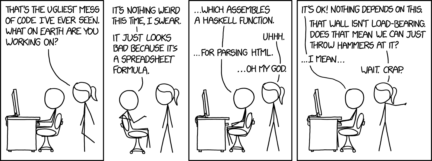
If your GenAI comes back with a program that you find difficult to understand - convoluted design, unclearly named objects, too many nested functions or loops, and so on - you will need to refactor the code so that it is easier to tweak and update.

2.7.3 Interpretable

Even if you use GenAI to produce code and/or analysis, ultimately the ownership of the project lies with you. It is extremely important that you understand, and are able to explain, the steps that the AI took; whether or not you directly performed them.

Note

In this course, the interpretable element is also how we define academic integrity.

We expect that any AI-produced content you include in your work to be something you can completely and correctly explain without the AI’s help.

If we suspect that AI is being overused in inappropriate ways - such as homework questions being copy-pasted into the prompt and the AI response being copy-pasted back with no oversight - we will address this by sitting down with you and asking you to explain the content step by step.

It is your responsibility to take the time and ensure you truly understand each task that you “outsource” to a GenAI tool.

2.7.4 Reproducible

We call a data analysis reproducible if it is structured and documented in such a way that it is easily repeatable with new data or by new researchers.

A current weakness of GenAI tools is that they often produce code that is too specifically tailored to the data given; code that cannot be generalized to the full data problem.

Consider, for example, the following suggestion from ChatGPT 4o, in response to the prompt “Write me a python program to find all the first names used in the lyrics of a given song.”

import re

# A list of common first names directly embedded in the script
FIRST_NAMES = {
    'John', 'Paul', 'Ringo', 'Mary', 'Lucy', 'David', 'Sarah', 'James',
    'Michael', 'Jennifer', 'Linda', 'Elizabeth', 'George', 'Emma',
    'Liam', 'Olivia', 'Noah', 'Ava', 'Sophia', 'Isabella'
    # Add more first names as needed
}

def find_first_names_in_lyrics(lyrics, first_names):
    """Find all first names in the given song lyrics."""
    # Split lyrics into words and remove punctuation using regex
    words = re.findall(r'\b\w+\b', lyrics.lower())
    
    # Find intersection of words in lyrics with the first names
    found_names = {word.capitalize() for word in words if word in first_names}
    
    return found_names

Here we see that the LLM suggests an approach of manually making a list of common first names. As you can imagine, this is unlikely to be the design that a data scientist would use. Not only does it require manually making a list of common names, or finding a resource like that online, this approach would miss uncommon first names. We would be more likely to use strategies like looking for capitalized words, sentence syntax, context, and so on.

The LLM’s approach would not be reproducible outside of the example songs it seems to have used to select 'John', 'Paul', 'Ringo', 'Mary', 'Lucy' as common names. (What songs could this be, do you think?)

When you generate code from an LLM, it is your responsibility to look for “hard-coded” or otherwise unreproducible elements of the program, and to instead implement a more generalizable approach.

2.7.5 Dependable

The simplest and most important question to ask about your AI-produced code or analysis is: is it correct?

If we have met the previous four guidelines, we know our output is: - Answering the right question - Possible to change if needed - Following a process we understand - Generalized, not hard-coded

But… does it actually achieve the desired task in a proper way?

It is not enough for you to be convinced that your procedure works. You need to provide solid reassurances of its dependability.

2.7.5.1 Unit testing

In programming, there is one way to do this: writing small unit tests that check whether your code outputs the values you wanted it to.

Unit tests can be a very structured and formal, like the code checks that automatically run when a developer updates a particular library, to make sure the updates didn’t cause a breaking change in the software. But they can also be quick and informal, like putting a few different inputs into your function to make sure it behaves how you expect.

Important

We cannot emphasize this enough: Unit tests are the best and most important way to prove to yourself, to us, and to your clients that the code you created (with or without AI) works the way you claim it does.

Practice Activity

Here is a conversation with ChatGPT 4o, in which it is asked to create a program to find all prime numbers in a certain range, and a program to find all perfect numbers in a certain range.

You may not understand every step of the code, nor the math procedure being used. That’s okay for this exercise.

Copy the code into a Colab Notebook. Then write a few unit tests that check if it works. Make sure to include some unexpected or unusual inputs, to try to “challenge” the program to break!

2.7.6 Even WEIRD-ER: Ethics and References

The WEIRD guidelines are focused on making sure the actual content and results of AI work is trustworthy.

Don’t forget, though, to be even WEIRD-ER: we also expect you to consider the Ethical issues of your AI use, and to thoroughly Reference any AI contribution to your work.

In every Lab Assignment, we expect an appendix with an Ethics Statement and References, both of which might need to reference your AI use.

An example ethics statement might look something like:

This analysis includes a comparison of male and female sex penguins. It therefore omits penguins with unknown sex or with unidentifiable biological sex. This analysis also makes use of Generative AI to suggest comparisons across penguin sex, and these tools may overlook exceptions to the sex binary.

An example reference statement including AI might look something like:

Chat-GPT 4o was used to suggest several analyses, including the Two-Way ANOVA test for body mass across sex and habitat. It was also used to generate first-draft code to perform this ANOVA test and create the corresponding boxplot.

2.7.7 Try it out

Practice Activity

Complete this activity with a partner.

This means that doubles take up more memory but can store more decimal places. You don’t need to worry about this in anything we will do.↩︎
In some ways, this is like the difference between an automatic and a manual transmission - you have fewer things to worry about, but you also don’t know what’s going on under the hood nearly as well↩︎
Throughout this section (and other sections), lego pictures are rendered using https://www.mecabricks.com/en/workshop. It’s a pretty nice tool for building stuff online!↩︎
Grumpy cat, Garfield, Nyan cat. Jorts and Jean: The initial post and the update (both are worth a read because the story is hilarious). The cats also have a Twitter account where they promote workers rights.↩︎